Download
1 / 52
630 likes | 1.05k Views
TFT(Thin Film Transistor) LCD II. Contents. TFT-LCD Overview Structure of TFT-LCD Panel (Back Light System, Polarizer, Color Filter) Pixel Structure TFT Fabrication TFT-LCD Driver (Data & Gate Driver) and Interface System Issues and Technologies of TFT-LCD High Gray Scale

E N D
Contents • TFT-LCD Overview • Structure of TFT-LCD Panel (Back Light System, Polarizer, Color Filter) • Pixel Structure • TFT Fabrication • TFT-LCD Driver (Data & Gate Driver) and Interface System • Issues and Technologies of TFT-LCD • High Gray Scale • Low Power Consumption • High Aperture Ratio • Wide Viewing Angle • Large Size Display
Gray Scale Generation • Various gray scale generation Methods • Decoder-BasedDAC • Resistor-String DAC • Capacitor DAC • Weighted Capacitance Type DAC • Split Weighted Capacitance Type DAC • C-2C Type DAC • Ramp Method • Dithering Method • FRC(Frame Rate Control) • Shindou Method
Digital Data Driver _Decoder Based DAC • DAC Using Decoder • Pros • Clear and fast operation • Relatively simple circuit • Cons • As many external voltage sources and analog switches as gray scales • Many voltage source : High system costs • Many analog switches : Large area • Impractical for high gray scale 3bit data V0 V1 V2 V3 V4 V5 V6 V7 Pass gate array Decoder 3-to-8 decoder based DAC
Digital Data Driver_Resistor String DAC • 8 bit Resistor String DAC • External voltage sources • 8-resistor string between neighboring voltage sources • 256 analog voltage levels • Pros • Less voltage sources than decoder-only type • More accurate than capacitor DAC • Cons • Static currents • Difficult to implement accurate resistance • Area increase with gray scale 8-bit resistor string DAC
16/15C - Vout + 4C 8C C 2C 4C 8C C 2C C Reset VREF1 VREF2 Digital Data Driver_Capacitor DAC • Capacitor DAC • Analog voltage generation controlling charge sharing between capacitors • Binary weighted capacitor • Pros • No static current • Less external voltages (1 or 2) • Easier to control thermal oxide thickness Uniform capacitors • Cons • Large area : DAC unit at every line • Variable data line capacitance • When OP-AMP not used • Less accurate than R-DAC
Reference voltages —D7 —D6 —D5 2C 2C 2C 2C VO Vr+ Vr- C C C C C C D0 D1 D2 D3 D4 Vr- Vr+ Digital Data Driver_C-2C DAC • 8-bit D/A Converter with -correction • Reference voltages can be adjusted to the LCD’s non-linear V-T characteristics • Small area of DAC compared with weighted capacitor type • Power consumption is reduced Reference voltage selector (upper 3-bit decoder) 5-bit C-2C DAC
Digital Data Driver_Ramp method Input register • DAC Using Ramp Signal : 6Bit • Structure • Shift register, Input register, Storage register, Counter, Analog switch • Externally supplied ramp signal • Operation • When a counter counts up to 111111, it turns-off the analog switch. • If an input data is 111111, the analog switch is turned-off as soon as the data is loaded • If an input data is 000000, the analog switch keeps being turned-on until the counter counts from 000000 to 111111. • The counter determines when to turn-off the switch Data Load Clock 5-bit counter External ramp External ramp Data= 000010 Data= 111101 Counter Output DAC Output
T(%) V7 Counter Output 000 001 010 011 100 101 110 111 100 Time V6 V1 80 V5 V2 V3 V4 60 V3 V3 V3 V2 40 External Ramp V2 V1 20 V1 V(volt) V0 0 1 2 3 4 5 Digital Data Driver_Ramp method • Cons • – Complex circuitry • ( 6bit counter at every data line ) • – Ramp signal distortion due to RC • delay and noise • Pros • – -correction by control of voltage • step V1, V2 , V3 (See below) • – No resistor, capacitor or amplifier • Better uniformity V-T nonlinearity compensation using ramp signal V-T characteristics of LC
Digital Data Driver_Dither method • Principles • V4 represents 12th gray, V5 represents 16th gray • Group 4 pixels as a unit • 4 pixels select 12th gray, 12th gray on average • 3 pixels select 12th gray, 13th gray on average • 2 pixels select 12th gray, 14th gray on average • 1 pixel select 12th gray, 15th gray on average • All pixels select 16th gray, 16th gray on average Driving Voltage and Gray Scale Gray Scale Interpolation using Dither-Method • Cons • Reduced resolution
Digital Data Driver_Frame Rate Control Gray Scale Using FRC 4-level V-T characteristics • Frame Rate Control - Temporal average • Cons • Should increase to prevent flicker • High speed addressing required unsuitable for high gray scale • Principle • V0, V1 alternation : • V0, V2 alternation :
m n Vi Vj Digital Data Driver_Shindou method[1/2] • Principle • Alternation of Vi, Vj of which duty ratio is m:n • Average voltage transferred to pixel • Controlling m and n : interpolation between Vi and Vj • Theoretical Background • An periodic function f(x) can be expressed in Fourier series • Data line and pixel act as a low pass filter • Harmonics are suppressed and DC (average value) component are transferred to pixel
Digital Data Driver_Shindou method[2/2] • Operation • SC selects neighboring two voltage sources according to higher 3bits D5, D6, D7. • ISG generates 32 kinds of pulse T whose duty ratios are 31:1~0:32 using TMs according to lower 5bits D0, D1, D2, D3, D4, D5. • The selected two voltage levels are interpolated by the generated pulse T Output Stage Using Shindou Method Structure of SCC Waveforms of TMs
Issues and Technologies for High Gray Scale • Issues • Vp compensation • Capacitor coupling structure • Vp compensation structure • Random offset of the output buffer • Offset compensation structure • Area Increases of the DAC • Compact DAC data driver (SID ’00) • New Driving Method for 8bit gray scale is needed
Vp problems • Vp problem(Gate Voltage Feedthrough)
Uneven parasitic capacitance in all pixels Asymmetric charging characteristic Uneven Vp in all pixels Degradation of gray scale Vp problems • What troubles in Vp ? • To reduce Vp • Pixel design optimization • Vp compensation circuit too complex • Novel methods are needed.
Vp Compensation Driving • LC voltage at the end of selection Vg,n Column Row n Vg,n CGS t Tr Vg,n-1 CST CLC Row n-1 Vg,n-1 Vcomp t
Difficult Random offset of the output buffer • Random Offset Process variations between channel-to-channel, chip-to-chip, wafer-to-wafer Without Offset Cancellation Technique Decrease of Yield With Offset Cancellation Technique
Random offset of the output buffer • Why Difficult ? • Different loads of OP-AMP • Calibration mode < 1pF • Driving mode > 100pF • Difficult to design OP-AMP • Solutions • OP-AMP with internal offset calibration • External offset calibration technique • Driving methods insensitive to offset voltage Common Offset Cancellation Circuit
Area Increases of the DAC • DAC • Resistor String DAC • Capacitor DAC etc. doubled DAC area (in resistor string DAC) 1-bit increase 8-bit DAC Area 10-bit DAC Area 4 times larger • Solutions • - New DAC schemes 8-bit DAC
Digital Data Driver_Area-efficient driver [1/2] Control Logic • Operation • Once the data are converted to parallel, they are fed into six DACs • The result is six analog voltages, which are multiplexed onto sample and hold cells, one for each output 36 6-Bit DAC (6 Stage) Data Vgamma 8 Analog Sample Circuit Analog Sample Circuit Analog Sample Circuit Analog Sample Circuit Analog Sample Circuit Analog Sample Circuit Analog Sample Circuit Analog Hold Circuit Analog Hold Circuit Analog Hold Circuit Analog Hold Circuit Analog Hold Circuit Analog Hold Circuit Analog Hold Circuit Buffer Buffer Buffer Buffer Buffer Buffer Buffer DRV OUT<1> DRV OUT<383> DRV OUT<2> DRV OUT<3> DRV OUT<384> DRV OUT<4> Compact(Area Efficient) LCD Driver
Digital Data Driver_Area efficient driver [2/2] • Pros • Area-efficient • 6bit * 384 DACs are needed for conventional data driver • 6bit * 6 DACs + 384 sample and hold circuits for compact driver • Low power consumption because of the reduced static currents of DACs • Cons • Sample and hold circuits errors are included (inapplicable to high gray scale)
Circuit Unit 40% Backlight Unit 60% Low Power Consumption • Overview Reduction of panel load driving power Improvement of transmission rate of panel • Panel load capacity reduction • Energy recovery driving • Reduced frame rate • Improvement of panel aperture ratio • High transmission rate color filters, • polarizers Low voltage drive circuits • 5V 3.3V Improvement of light utilization rate Excellent-efficiency power supply circuit • Efficiency improvement of light • guides • Improvement of light emission • efficiency of CCFT • Efficiency improvement of • DC/DC converter
Panel AC Power Analog DC Power Interface Bus Power Digital Power Power Breakdown of Data Driver Power Consumption (12.1 inch SVGA ,SID ’97)
Low Power Driving(AC Power Reduction) • Equation of the Panel AC Power Consumption • Two approaches to reduce AC power Reduce FROW Reduce VSWING • MFD(Multi-Field Driving) • Charge Sharing • Triple Charge Sharing • Stepwise Source Driving • RLC Resonant Method
Low Power Driving - Multi-Field Driving [1/3] • Background • Total power consumption (TPC) = Static power consumption (SPC)+Dynamic Power Consumption (DPC) • DPC is 70% of TPC, so refresh rate must be slow down for TPC reduction, because DPC is directly proportional to refresh rate • Slower refresh rate causes more visible flicker! Multi-Field Driving • Multi-Field Driving Method • Divide 1 frame into 3 sub-field • The polarity of adjacent field is opposite • In spite of reduced refresh rate, Flicker frequency remains at the same level due to averaging effect
Low Power Driving - Multi-Field Driving [2/3] • Flicker Compensation • In the case that refresh rate is reduced from 60Hz to 20Hz • Flicker frequency for each line : 2TS (three times longer than original one) • Flickers for adjacent three lines occur at different phase • Average flicker frequency for three serial lines : 2/3 TS In spite of reducing refresh rate into 1/3 of original one, flicker frequency remains at the same level (a) Flicker for one line (b) Flicker for adjacent three lines (C) Average flicker for adjacent three lines
Low Power Driving - Multi-Field Driving [3/3] • Power Consumption Reduction • Pros. • - power saving efficiency > 50% • Cons. • - Inapplicable to moving image • - extra frame memory • - complex
Low Power Driving - Charge Sharing [1/2] Waveform and timing diagram • Operation • Now Mth row was driven and (M+1)th row is about to be driven • Neighboring data lines store video signals of opposite polarities • Shortly before driving Mth row, every switch is disconnected from output buffer and connected to CL • Every data line has medium voltage level due to charge sharing • Signal CR controls the switches Architecture
Low Power Driving - Charge Sharing [2/2] • Power Consumption Analysis • Vpos voltage level of video signal of positive polarity • Vneg voltage level of video signal of negative polarity • Half of Vswing is supplied by charge sharing and only the other half comes from the external source • Pros. • - applicable to moving image • - no degradation of image quality • - very simple • - power saving efficiency < 50% • Cons. • - power saving efficiency < 50%
Low Power Driving - Triple Charge Sharing [1/3] Architecture Waveform and Timing Diagram
Low Power Driving - Triple Charge Sharing [2/3] • Convergence of the voltage of CEXT If after thousands of row line time
Low Power Driving - Triple Charge Sharing [3/3] Power consumed in Gray Scale Decision Time : • Pros. • - applicable to moving image • - no degradation of image quality • - simple • - power saving efficiency < 66.6% • Cons. • - row line time extension method • is needed
Voltage swing A B C D Power supply amplifier Power supply Polarity modulator VL Polarity modulator VH amplifier amplifier Low Power Driving - Stepwise Source Driving [1/3] Conventional Source Driving Stepwise Source Driving
Low Power Driving - Stepwise Source Driving [2/3] • Schematic Diagram Polarity Modulator Architecture of Driver
Low Power Driving - Stepwise Source Driving [3/3] • Pros. - applicable to moving image - no degradation of image quality - power saving efficiency < 84.5% • Cons. - row line time extension method is needed - voltage overcharging Waveform in All-Black image Waveform in All-White image
L Low Power Gate Driving_RLC Resonant Method [1/2] • Operation • RLC resonant operation whose oscillation is interrupted after half oscillation • Oscillation sensing circuitry sense the ON-resistance of the switch - + VS/2 CL Simplified Structure Schematic View of Driving Circuitry
Low Power Gate Driving_RLC Resonant Method [2/2] • Operation time range • Charging (discharging) time is divided into two oscillation time and two charge sharing time • Power dissipation • Applicable to gate and data driver of LCD Timing diagram
VDD Vos1 Cmp1 Vout Vin Vos2 Cmp2 VSS Low Analog DC Power_Class-B Buffer • Operation • Nonlinear circuits are included (inverter and comparator) • Output NMOS and PMOS are turned on by series-shunt feedback of input/output voltage • Pros • Low static current • Cons • Sensitive to the offset voltage of comparators Block diagram of class-B output buffer
High Aperture Ratio TFT • Aperture ratio decreases as pixel pitch shrinks • Use of Black matrix • Prevent light transmittance through a pixel surrounding area • High aperture ratio structure • Shield CS(storage capacitor) structure • ITO Shield Plane structure Gate Line Black matrix Data Line Storage Capacitance Aperture Area Aperture of a Single Pixel
High Aperture Ratio • Shield-CS structure • Shield-CS pattern(electro-static layer) functions as a common electrode of a storage capacitance • Coupling capacitance between the signal line and the pixel electrode can be reduced • This permits close layout between signal electrode and the pixel electrode • ITO-shield plane structure • Transparent electrode is placed between the signal line and the pixel electrode • This electrode works as a ground plane and shields capacitive coupling • Transverse electric field is reduced due to the same reason as the shield CS
High Aperture Ratio Aperture Area Alginment margin Conventional Structure Black Matrix Signal Line Aperture Area No Black Matrix Signal Line Alginment margin Shield -CS Pixel Electrode Shield Cs Shield and storage capacitance electrode Liquid Crystal ITO Shield Plane Insulator Signal Line
High Aperture Ratio Black matrix CS Conventional Structure Aperture area Shield -CS ITO Shield Plane 50 ~ 70% 70 ~ 80% 80 ~ 90%
Wide Viewing Angle • Conventional TN Structure • Anisotropic Structure of LC molcule • Imperfect light control (Use of Polarizer) • Viewing angle dependence is intrinsic problem of LCD • Gray scale inversion occurrs Viewing Angle 90°(H), 40°(V) Aperture Ratio 50~70%
Wide Viewing Angle • Vertical Alignment Mode • Advantages • Wide viewing angle without gray scale inversion • High contrast ratio(~300:1) • Fast response time(~25ms) • Disadvantages • Material Limitation(LC) • Use of compensation film • Adoption of multi-domain technology • Complicate LC process • Unstable alignment to mechanical shock Viewing Angle 140°(H), 120°(V) Aperture Ratio > 80%
Wide Viewing Angle • In-Plane Switchig • Advantages • Wide viewing angle without gray scale inversion • Low flicker level(Unvisible) • Low cost • Disadvantages • Slow response time(>45ms) • Low transmittance(<4%) • Crosstalk • High driving voltage Viewing Angle 160°(H), 160°(V) Aperture Ratio< 40%
Large Panel Size and High-Resolution • Issues • Shortage of the Row Line Time • Solutions • Dual Line Scanning • Display Area Division Scanning • LiTEX(Line Time Extension)
Large-Size High -Resolution Increase of parasitic loads Increase of RC charging time Decrease of row line time Deterioration of Image Quality Needs for Increase techniques of row line time Row Line Time and Resolution 35 30 25 20 XGA SXGA UXGA QXGA Row Line Time (sec) 15 10 5 0 50 55 60 65 70 75 80 Frame Rate(Hz)
Effective Mobility and Resolution • Effective mobility : minimum mobility necessary to achieve the maximum aperture ratio • Effective mobility is increased as panel size is larger • Effective mobility is increased as the resolution of panel is higher 2.5 XGA SXGA UXGA QXGA Effective mobility (Cm2/vs) 2.0 1.5 1.0 0.5 0.0 200 300 150 250 Pixel Pitch (m)
Dual Line Scanning Method • Dual Line Scanning Method • Pros. : Doubled Row Line Time • Cons. : Decrease of Vertical Resolution (1/2 of conventional) • Display-Area division scanning • Pros. : Doubled Row Line Time • Cons. : Cost Increase (Doubled Driver LSIs)