Download
1 / 40
400 likes | 575 Views
More on Indexes. Secondary Indexes B-Trees. Source: our textbook, slides by Hector Garcia-Molina. Secondary Indexes. Sometimes we want multiple indexes on a relation. Ex: search Candies(name,manf) both by name and by manufacturer

E N D
More on Indexes Secondary Indexes B-Trees Source: our textbook, slides by Hector Garcia-Molina
Secondary Indexes • Sometimes we want multiple indexes on a relation. • Ex: search Candies(name,manf) both by name and by manufacturer • Typically the file would be sorted using the key (ex: name) and the primary index would be on that field. • The secondary index is on any other attribute (ex: manf). • Secondary index also facilitates finding records, but cannot rely on them being sorted
Sparse Secondary Index? • No! • Since records are not sorted on that key, cannot predict the location of a record from the location of any other record. • Thus secondary indexes are always dense.
30 20 80 100 90 40 70 10 60 50 90 30 ... 20 80 100 does not make sense! Sequence field • Sparse index
Design of Secondary Indexes • Always dense, usually with duplicates • Consists of key-pointer pairs ("key" means search key, not relation key) • Entries in index file are sorted by key • Therefore second-level index is sparse
90 30 20 80 100 50 70 40 10 60 50 10 10 20 50 60 30 70 90 40 ... ... sparse second- level Secondary indexes Sequence field dense first- level
Secondary Index and Duplicate Keys • Scheme in previous diagram wastes space in the present of duplicate keys • If a search key value appears n times in the data file, then there are n entries for it in the index.
30 20 20 10 10 10 40 40 40 40 40 10 20 10 30 40 10 40 ... 20 40 Duplicate values & secondary indexes one option... • Problem: • excess overhead! • disk space • search time
Buckets • To avoid repeating values, use a level of indirection • Put buckets between the secondary index file and the data file • One entry in index for each search key K; its pointer goes to a location in a "bucket file", called the bucket for K • Bucket holds pointers to all records with search key K
10 30 20 20 10 10 40 40 40 40 50 10 20 60 ... 30 40 Duplicate values & secondary indexes saves space as long as search-keys are larger than pointers and average key appears at least twice buckets
Why “bucket” idea is useful Indexes Records name: primary Emp (name,dept,floor,...) dept: secondary floor: secondary
Query: SELECT name FROM Emp WHERE dept = 'Toy' AND floor = 2 dept index Emp floor index Toy 2 • Intersect Toy dept bucket and floor 2 bucket to get set of matching Emp’sSaves disk I/O's
Summary of Indexes So Far • Advantages: • simple • index is sequential file, good for scans • Disadvantages • either inserts are expensive • or lose sequentiality (cf. next slide) • Instead use B-tree data structure to implement index
32 39 38 31 33 34 35 36 overflow area (not sequential) 10 20 30 Example Index (sequential) continuous free space 40 50 60 70 80 90
B-Trees • Several related data structures • Key features are: • automatically adjust number of levels of indexes as size of data file changes • storage on blocks is managed to keep every block between half full and full => no overflow blocks needed • We'll actually study B+ trees
B-Tree Structure • an example of a balanced search tree: every root-to-leaf path has same length • each node (vertex) in the tree is a block, which contains search keys and pointers • parameter n, which is largest value so that n+1 pointers and n keys fit in one block • Ex: If block size is 4096 bytes, keys are 4 bytes, and pointers are 8 bytes, then n = 340.
Constraints on B-Tree Nodes • Keys in leaf nodes are copies of keys from data file, in sorted order • Root contains between 2 and n+1 index node pointers • Each internal node contains between (n+1)/2 and n+1 index node pointers • Each non-leaf node consists of ptr1,key1,ptr2,key2,…,keym-1,ptrm where ptri points to index node with keys between keyi-1 and keyi
Constraints (cont'd) • Each leaf contains between (n+1)/2 and ndata record pointers, plus a "next leaf" pointer • Associated with each data record pointer is a key, and the pointer points to the data record with that key
Example B-tree nodes with n = 3 more concise notation textbook notation 30 35 30 Leaf: 35 to record with key 30 to record with key 35 30 30 Non-leaf: to part of tree with keys < 30 to part of tree with keys ≥ 30
Sample non-leaf 57 81 95 to keys to keys to keys to keys < 57 57 k<81 81k<95 95
Sample leaf node: From non-leaf node to next leaf in sequence 57 81 95 To record with key 57 To record with key 81 To record with key 85
n=3 Full node min. node Non-leaf Leaf 120 150 180 30 3 5 11 30 35 counts even if null
B-Tree Example n=3 100 Root 120 150 180 30 3 5 11 120 130 180 200 100 101 110 150 156 179 30 35 … to records …
Insert into B+tree (a) simple case • space available in leaf (b) leaf overflow (c) non-leaf overflow (d) new root
32 n=3 100 (a) Insert key = 32 30 3 5 11 30 31
7 3 5 7 n=3 100 (a) Insert key = 7 30 3 5 11 30 31
160 180 160 179 n=3 100 (c) Insert key = 160 120 150 180 180 200 150 156 179
30 new root 40 40 45 n=3 (d) New root, insert 45 10 20 30 1 2 3 10 12 20 25 30 32 40
Deletion from B-tree (a) Simple case - no example (b) Coalesce with neighbor (sibling) (c) Re-distribute keys (d) Cases (b) or (c) at non-leaf
40 n=4 (b) Coalesce with sibling • Delete 50 10 40 100 10 20 30 40 50
35 35 n=4 (c) Redistribute keys • Delete 50 10 40 100 10 20 30 35 40 50
new root 40 25 30 (d) Non-leaf coalese • Delete 37 n=4 25 10 20 30 40 25 26 30 37 1 3 10 14 20 22 40 45
B-tree deletions in practice • Often, coalescing is not implemented • Too hard and not worth it!
Applications of B-Trees • B-tree is used to implement indexes • The data record pointers in the leaves correspond to the data record pointers in sequential indexes • Some example uses: • B-tree search key is primary key for data file, leaf pointers form a dense index on the file • B-tree search key is primary key for data file, leaf pointers form a sparse index on the file • B-tree search key is not primary key, leaf pointers form a dense index on the file
B-Trees with Duplicate Keys Change definition of B-tree: • If key K appears in an internal node, then K is the smallest "new" key in the subtree S rooted at the pointer that follows K in the node • "New" means K does not appear in the part of the B-tree to the left of S but it does appear in S • Allow null key in certain situations
Example B-Tree with Duplicates 17 -- 37 43 7 2 3 5 23 23 43 47 13 17 23 23 37 41 7 13
Lookup in B-Trees • Assume no duplicate keys. • Assume B-tree is a dense index. • To find the record with key K, search starting at the root and ending at a leaf: • if current node is not a leaf and has keys K1, K2, …, Kn, find the smallest key, Ki, in the sequence that is ≤ K. • follow the (i+1)-st pointer to a node at the next level and repeat • when a leaf node is reached, find the key with value K and follow the associated pointer to the data record
Range Queries with B-Trees • Range query: a query in which a range of values is sought. Examples: • SELECT * FROM R WHERE R.k > 40; • SELECT * FROM R WHERE R.k >= 10 AND R.k <= 25; • To find all keys in the range [a,b]: • Do a lookup on a: leads to leaf where a could be • Search the leaf for all keys ≥ a • If we find a key > b, we are done • Else follow next-leaf pointer and continue searching in the next leaf • Continue until finding a key > b or no more leaves
Efficiency of B-Trees • B-trees allow lookup, insertion and deletion of records with very few disk I/Os • Number of disk I/Os is number of levels in the B-tree plus cost of any reorganization • If n is at least 10, then splitting/merging blocks will be rare and usually limited to the leaves • For typical sizes of keys, pointers, blocks and files, 3 levels suffice (see next slide) • Also can keep root block of B-tree in memory
Size of B-Tree • Assume • 4096 bytes per block • 4 bytes per key (e.g., integer) • 8 bytes per pointer • no header info in the block • Then n = 340 (can keep n keys and n+1 pointers in a block) • Assume on average a block has 255 pointers • Count: • one node at level 1 (the root) • 255 nodes at level 2 • 255*255 = 65,025 nodes at level 3 (leaves) • each leaf has 255 pointers, so total number of records is more than 16 million