Download
1 / 49
620 likes | 899 Views
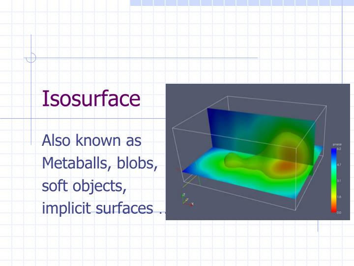
Isosurface. Also known as Metaballs, blobs, soft objects, implicit surfaces …. Outline. Marching cube algorithm Isosurface Metaballs Implicit modeling Volume rendering. Introduction. iso -surface: equal. Surface-based visualization technique for scalar data field

E N D
Isosurface Also known as Metaballs, blobs, soft objects, implicit surfaces …
Outline • Marching cube algorithm • Isosurface • Metaballs • Implicit modeling • Volume rendering
Introduction iso-surface: equal • Surface-based visualization technique for scalar data field • treat isosurface as one special instance of implicit function: f(x,y,z) = c • Prevailing technology: marching cube (patented) • Related: marching tetrahedra
Basic Idea(Marching Square) References: 1, 2 value = 5
Continuation: O(n2) function evaluations Need a starting point for each piece of disjoint surface Designed for continuous, real-valued functions Exhaustive search: O(n3) function evaluations Can find all pieces of surfaces Designed to process 3D arrays (CT, MRI) Continuation vs. Exhaustive Search (3D)
Similar ambiguity can occur Need to resolve the topological inconsistency (more cases devised; see reference) Marching Cube
Determining normals at vertices of triangular faces • It is often necessary to create normals for each vertex of the triangular faces for smooth shading. • After the facets have been created, compute the average of the normals of all the faces that share a triangle vertex. • A common approach is at each vertex to use a weighted average of normals of the polygons sharing the vertex. The weight is the inverse of the area of the polygon, so small polygons have greater weight. The idea is that small polygons may occur in regions of high surface curvature. • The original Siggraph paper computes normals at vertices by interpolating the normals at the cube vertices. These cube vertex normals are computed using Central Differences of the volumetric data.
Grid Resolution • One very desirable control when polygonizing a field where the values are known or can be interpolated anywhere in space is the resolution of the sampling grid. This allows coarse or fine approximation to the isosurface to be generated depending on the smoothness required and/or the processing power available to display the surface.
Marching Tetrahedra Decompose a cube into six tetrahedra • Jules Bloomenthal (Graphics Gems IV)
MT (cont) • Pros • No ambiguous cases • simpler implementation • Cons • Number of triangles quality of triangles • Shirley90 decomposes a cube into 5 tetrahedra (smallest number of tetrahedra possible)
Regularized MT (Treece98) • MT: overcome topological problem (false positive/false negative) of MC • But problem still exists: poor triangle quality; MT has many triangles • “regularized”: combine with vertex clustering (but still maintain topological property) result: good fewer triangles
MC Codes • References and codes for marching cube and marching tetrahedra are on Paul Bourke’s page
A Brief History (ref) • People have known for a long time that if you have two implicit surfaces f(x,y,z)=0 and g(x,y,z)=0 that are fairly continuous, with a common sign convention (f and g positive on the inside, negative on the outside, say) then the implicit surface defined by f+g=0 is a blend of the shapes. See [Ricci 1983] for a variant of this. The van der Waals surfaces of molecules (roughly speaking, iso-potentials of the electron density) are described in Chemistry and Physics books and [Max 1983]. To create animation of DNA for Carl Sagan's COSMOS TV Series, Jim Blinn proposed approximating each atom by a Gaussian potential, and using superposition of these potentials to define a surface. He ray traced these [Blinn 1982], and called them "blobby models". • Shortly thereafter, people at Osaka University and at Toyo Links in Japan began using blobby models also. They called theirs "metaballs" (or, when misspelled, "meatballs"). Yoichiro Kawaguchi became a big user of their software and their Links parallel processor machine to create his "Growth" animations which have appeared in the SIGGRAPH film show over the years. The graduate students implementing the metaball software under Koichi Omura at Osaka used a piecewise quadratic approximation to the Gaussian, however, for faster ray-surface intersection testing (no need for iterative root finders; you just solve a quadratic). I don't know of any papers by the Japanese on their blobby modeling work, which is too bad, because they have probably pushed the technique further than anyone. • Bloomenthal has discussed techniques for modeling organic forms (trees, leaves, arms) using blobby techniques [Bloomenthal 1991] (though he prefers the term "implicit modeling") and for polygonizing these using adaptive, surface- tracking octrees [Bloomenthal 1988]. The latter algorithm is not limited to blobby models, but works for any implicit model, not just blobs. Polygonization allows fast z-buffer renderers to be used instead of ray tracers, for interactive previewing of shapes. A less general variant of this algorithm was described in the "marching cubes" paper by [Lorensen 87] and some bugs in this paper have been discussed in the scientific visualization community in the years since. In the sci-vis community, people call them "iso-surfaces" not "implicit surfaces". • Meanwhile, in Canada and New Zealand, the Wyvill brothers, and grad students, were doing investigating many of the same ideas: approximations of Gaussians, animation, and other ideas. See their papers listed below. Rather than "blobbies" or "metaballs", they called their creations "soft objects". But it's really the same idea. • Bloomenthal and Wyvill collected many good papers on blobby and implicit modeling for a recent SIGGRAPH tutorial (1991?).
Metaball Modeling • Each metaball as a positively charged particle, with a suitable (differentiable) potential function • Implicit function f(x,y,z): the potential field formed by summing contribution of all metaballs • Rendering isosurfaces • Surface-based: evaluate the potential at grid points; use marching cube • Ray-casting: for each ray, find the point of intersection (and corresponding normal for Phong shading)
Remark • The influence of each charged particle is negligible outside the 1/sqrt(2) concept of “bounding sphere” • When casting a ray, only find the metaballs that are active • For all the active metaballs along a ray, inch along the ray, sum up all active balls to find out the exact point (if any) where the potential exceeds the threshold • Determine the normal at such points by summing up the normal vectors of the active balls
Threshold zero More Rendering • Texture coordinate generation • Material …
35 metaballs Levels of control Mid: thigh, chest, … High: weight, sex, age, muscle, … Human Modeling Using Metaballs
Do not evaluate each cell Start from each ball, move along one direction until it reaches the “boundary” If the cell is not yet evaluated, do so and propagate to its adjacent cells MC Speed Up specifically for Metaballs (Ref)
Related: Implicit Modeling F(x,y,z) = c • F(x,y,z) = x2 + y2 + z2 − R2 • Simple geometric description (plane, spheres, cylinders, …) • Region separation • Can be combined to create complex objects using Boolean operators
Implicit Modeling To create CSG objects At a point x0,y0,z0 the value of • F G = min(F(x0,y0,z0), G(x0,y0,z0)) • F G = max(F(x0,y0,z0), G(x0,y0,z0)) • F − G = max(F(x0,y0,z0), −G(x0,y0,z0)) F(x,y)=x2+y2 − 22 G(x,y)=(x-3)2+(y-2)2 − 32 F G = 0
512x512x12-bit, upto 50 slices in a stack Each slice is spaced 1-5mm apart Volume Rendering
Example Jaw without skin Jaw with skin
Related Work • Iso-surface extraction • Implicit surface/metaballs • Thresholded data (medical imaging) • Surface from cross-sections