Lecture 12: Laplace Transform

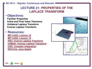
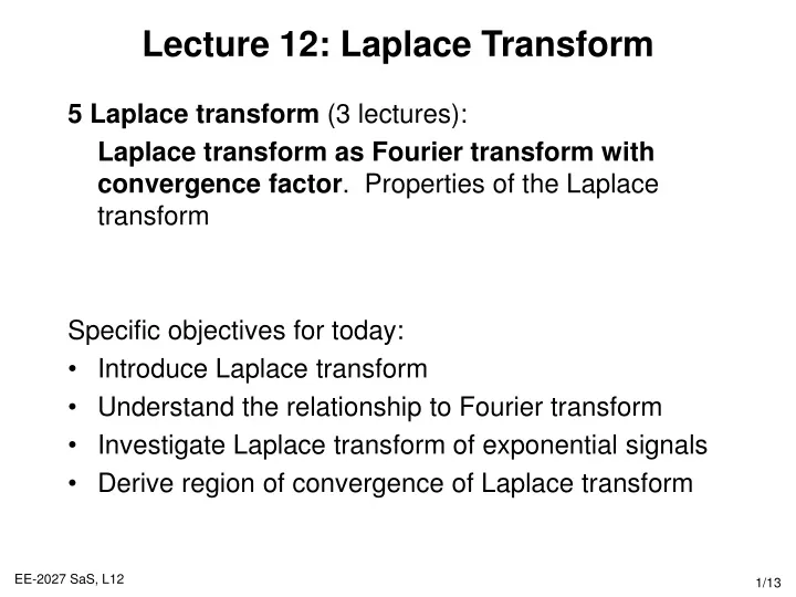
1. Lecture 12: Laplace Transform • 5 Laplace transform (3 lectures): • Laplace transform as Fourier transform with convergence factor. Properties of the Laplace transform • Specific objectives for today: • Introduce Laplace transform • Understand the relationship to Fourier transform • Investigate Laplace transform of exponential signals • Derive region of convergence of Laplace transform

2. Lecture 12: Resources • Core material • SaS, O&W, Chapter 9.1&9.2 • Recommended material • MIT, Lecture 17 • Note that in the next 3 lectures, we’re looking at continuous time signals (and systems) only

3. Introduction to the Laplace Transform • Fourier transforms are extremely useful in the study of many problems of practical importance involving signals and LTI systems. • purely imaginary complex exponentials est, s=jw • A large class of signals can be represented as a linear combination of complex exponentials and complex exponentials are eigenfunctions of LTI systems. • However, the eigenfunction property applies to any complex number s, not just purely imaginary (signals) • This leads to the development of the Laplace transform where s is an arbitrary complex number. • Laplace and z-transforms can be applied to the analysis of un-stable system (signals with infinite energy) and play a role in the analysis of system stability

4. The Laplace Transform • The response of an LTI system with impulse response h(t) to a complex exponential input, x(t)=est, is • where s is a complex number and • when s is purely imaginary, this is the Fouriertransform, H(jw) • when s is complex, this is the Laplace transform of h(t), H(s) • The Laplace transform of a general signal x(t) is: • and is usually expressed as:

5. Laplace and Fourier Transform • The Fourier transform is the Laplace transform when s is purely imaginary: • An alternative way of expressing this is when s = s+jw • The Laplace transform is the Fourier transform of the transformed signal x’(t) = x(t)e-st. Depending on whether s is positive/negative this represents a growing/negative signal

6. Example 1: Laplace Transform • Consider the signal • The Fourier transform X(jw) converges for a>0: • The Laplace transform is: • which is the Fourier Transform of e-(s+a)tu(t) • Or • If a is negative or zero, the Laplace Transform still exists

7. Example 2: Laplace Transform • Consider the signal • The Laplace transform is: • Convergence requires that Re{s+a}<0 or Re{s}<-a. • The Laplace transform expression is identical to Example 1 (similar but different signals), however the regions of convergence of s are mutually exclusive (non-intersecting). • For a Laplace transform, we need both the expression and the Region Of Convergence (ROC).

8. Example 3: sin(wt)u(t) • The Laplace transform of the signal x(t) = sin(wt)u(t) is:

9. Fourier Transform does not Converge … • It is worthwhile reflecting that the Fourier transform does not exist for a fairly wide class of signals, such as the response of an unstable, first order system, the Fourier transform does not exist/converge • E.g. x(t) = eatu(t), a>0 • does not exist (is infinite) because the signal’s energy is infinite • This is because we multiply x(t) by a complex sinusoidal signal which has unit magnitude for all t and integrate for all time. Therefore, as the Dirichlet convergence conditions say, the Fourier transform exists for most signals with finite energy

10. Im Im -a -a Re Re Region of Convergence • The Region Of Convergence (ROC) of the Laplace transform is the set of values for s (=s+jw) for which the Fourier transform of x(t)e-st converges (exists). • The ROC is generally displayed by drawing separating line/curve in the complex plane, as illustrated below for Examples 1 and 2, respectively. • The shaded regions denote the ROC for the Laplace transform

11. Example 4: Laplace Transform • Consider a signal that is the sum of two real exponentials: • The Laplace transform is then: • Using Example 1, each expression can be evaluated as: • The ROC associated with these terms are Re{s}>-1 and Re{s}>-2. Therefore, both will converge for Re{s}>-1, and the Laplace transform:

12. Lecture 12: Summary • The Laplace transform is a superset of the Fourier transform – it is equal to it when s=jw i.e. F{x(t)} = X(jw) • Laplace transform of a continuous time signal is defined by: • And can be imagined as being the Fourier transform of the signal x’(t) = x(t)est, when s=s+jw • The region of convergence (ROC) associated with the Laplace transform defines the region in s (complex) space for which the Laplace transform converges. • In simple cases it corresponds to the values for s (s) for which the transformed signal has finite energy

13. Questions • Theory • SaS, O&W, Q9.1-9.4, 9.13 • Matlab • There are laplace() and ilaplace() functions in the Matlab symbolic toolbox • >> syms a w t s • >> laplace(exp(a*t)) • >> laplace(sin(w*t)) • >> ilaplace(1/(s-1)) • Try these functions to evaluate the signals of interest • These use the symbolic integration function int()