BCOR 1020 Business Statistics

1. BCOR 1020Business Statistics Lecture 2 – January 17, 2008

2. Overview • Chapter 2 – Data Collection… • Key Definitions • Level of Measurement • Time Series vs. Cross-Sectional Data • Sampling Concepts • Sampling Methods • Data Sources • Survey Research

3. Chapter 2 – Key Definitions • Data is the plural form of the Latin datum (a “given” fact). • In scientific research, data arise from experiments whose results are recorded systematically. • In business, data usually arise from accounting transactions or management processes. • Important decisions may depend on data. • We will refer to Data as plural and data set as a particular collection of data as a whole. • Observation – each data value. • Subject(or individual) – an item for study (e.g., an employee in your company). • Variable – a characteristic about the subject or individual (e.g., employee’s income).

4. Chapter 2 – Key Definitions Three types of data sets:

5. Chapter 2 – Key Definitions Consider the multivariate data set with 5 variables 8 subjects 5 x 8 = 40 observations Multivariate data sets can become quite large.

6. Types of Data Attribute(qualitative) Numerical(quantitative) Verbal LabelX = economics(your major) CodedX = 3(i.e., economics) DiscreteX = 2(your siblings) ContinuousX = 3.15(your GPA) Chapter 2 – Key Definitions • A data set may have a mixture of data types.

7. Chapter 2 – Key Definitions Attribute Data: • Also called categorical, nominal or qualitative data. • Values are described by words rather than numbers. • For example, - Automobile style (e.g., X = full, midsize, compact, subcompact).- Mutual fund (e.g., X = load, no-load). Data Coding: • Coding refers to using numbers to represent categories to facilitate statistical analysis. (We need numerical representations to perform the math.) • Coding an attribute as a number does not make the data numerical. • For example, 1 = Bachelor’s, 2 = Master’s, 3 = Doctorate • Rankings may exist (consider the above example)

8. Chapter 2 – Key Definitions Binary Data – An Important Class of Attribute Data: • A binary variable has only two values, 1 = presence, 0 = absence of a characteristic of interest (codes themselves are arbitrary). • For example, 1 = employed, 0 = not employed 1 = married, 0 = not married 1 = male, 0 = female 1 = female, 0 = male • The coding itself has no numerical value so binary variables are attribute data.

9. Chapter 2 – Key Definitions Numerical Data – Numerical or quantitative data arise from counting, measurement or some kind of mathematical operation. • For example, • Number of auto insurance claims filed in March. • Length of time between customer arrivals on a webpage. • Ratio of profit to sales for last quarter. • Can be broken down into two types – discrete or continuous data.

10. Chapter 2 – Key Definitions Discrete Data – A numerical variable with a countable number of values that can be represented by an integer (no fractional values). • For example, • Number of Medicaid patients (e.g., X = 2). • Number of takeoffs at O’Hare (e.g., X = 37). Continuous Data – A numerical variable that can have any value within an interval (e.g., length, weight, time, sales, price/earnings ratios). • Any continuous interval contains infinitely many possible values (e.g., 426 < X < 428).

11. Clickers What type of data (attribute, discrete numerical, or continuous numerical) is your GPA? A = attribute B = discrete numerical C = continuous numerical

12. Clickers What type of data (attribute, discrete numerical, or continuous numerical) is the occupation of a mortgage applicant? A = attribute B = discrete numerical C = continuous numerical

13. Chapter 2 – Level of Measurement There are four levels of measurement for data:

14. Chapter 2 – Level of Measurement Nominal Measurement–Nominal data merely identify a category. Nominal data are qualitative, attribute, categorical or classification data (e.g., Apple, Compaq, Dell, HP). • Nominal data are usually coded numerically, codes are arbitrary (e.g., 1 = Apple, 2 = Compaq, 3 = Dell, 4 = HP). • Only mathematical operations are counting (e.g., frequencies) and simple statistics. Ordinal Measurement – Ordinal data codes can be ranked (e.g., 1 = Frequently, 2 = Sometimes, 3 = Rarely, 4 = Never). • Distance between codes is not meaningful (e.g., distance between 1 and 2, or between 2 and 3, or between 3 and 4 lacks meaning). • Many useful statistical tests exist for ordinal data. Especially useful in social science, marketing and human resource research.

15. Chapter 2 – Level of Measurement Interval Measurement – Data can not only be ranked, but also have meaningful intervals between scale points (e.g., difference between 60F and 70F is same as difference between 20F and 30F). • Since intervals between numbers represent distances, mathematical operations can be performed (e.g., average). • Zero point of interval scales is arbitrary, so ratios are not meaningful (e.g., 60F is not twice as warm as 30F).

16. Chapter 2 – Level of Measurement Likert Scales – A special case of interval (?) data frequently used in survey research. • The coarseness of a Likert scale refers to the number of scale points (typically 5 or 7). • A neutral midpoint (“Neither Agree Nor Disagree”) is allowed if an odd number of scale points is used or omitted to force the respondent to “lean” one way or the other. • Likert data are coded numerically (e.g., 1 to 5) but any equally spaced values will work. • Careful choice of verbal anchors results in measurable intervals (e.g., the distance from 1 to 2 is “the same” as the interval, say, from 3 to 4). • Ratios are not meaningful (e.g., here 4 is not twice 2). • Many statistical calculations can be performed (e.g., averages, correlations, etc.).

17. Chapter 2 – Level of Measurement Likert Scales – Example • Two variants of Likert scales…

18. Chapter 2 – Level of Measurement Ratio Measurement– Ratio data have all properties of nominal, ordinal and interval data types and also possess a meaningful zero (absence of quantity being measured). • Because of this zero point, ratios of data values are meaningful (e.g., $20 million profit is twice as much as $10 million). • Zero does not have to be observable in the data, it is an absolute reference point. Changing Data by Recoding – In order to simplify data or when exact data magnitude is of little interest, ratio data can be recoded downward into ordinal or nominal measurements (but not conversely). • For example, recode systolic blood pressure as “normal” (under 130), “elevated” (130 to 140), or “high” (over 140). • The above recoded data are ordinal (ranking is preserved) but intervals are unequal and some information is lost.

19. Chapter 2 – Level of Measurement Use the following procedure to recognize data types:

20. Clickers Which type of data (nominal, ordinal, interval, or ratio) is the pay of employees in the Wal-Mart store in Hutchinson Kansas? A = nominal B = ordinal C = interval D = ratio

21. Chapter 2 – Time Series & Cross-Sectional Data Time Series Data – Each observation in the sample represents a different equally spaced point in time (e.g., years, months, days). • Periodicity may be annual, quarterly, monthly, weekly, daily, hourly, etc. • We are interested in trends and patterns over time (e.g., annual growth in consumer debit card use from 1999 to 2006). Cross-sectional Data – Each observation represents a different individual unit (e.g., person) at the same point in time (e.g., monthly VISA balances). • We are interested in variation among observations or in relationships. • We can combine the two data types to get pooled cross-sectional and time series data.

22. Clickers Which type of data (time series or cross- sectional) is Mexico’s GDP for the last 10 quarters? A = time series B = cross-sectional

23. Chapter 2 – Sampling Concepts Sample or Census? • A sample involves looking only at some items selected from the population. • A census is an examination of all items in a defined population. • Why collect a sample rather than complete a census?

24. Chapter 2 – Sampling Concepts Situations Where A Sample May Be Preferred: • Infinite Population – Destructive Testing • Timely Results – Cost • Accuracy – Sensitive Information Situations Where A Census May Be Preferred: • Small Population – Large Sample Size • Database Exists – Legal Requirements

25. Chapter 2 – Sampling Concepts Parameters and Statistics: • Parameters – Any measurement that describes an entire population. Usually, the parameter value is unknown since we rarely can observe the entire population. Parameters are often (but not always) represented by Greek letters. • Statistics – Any measurement computed from a sample. Usually, the statistic is regarded as an estimate of a population parameter. Sample statistics are often (but not always) represented by Roman letters. Sample (Size = n): Statistics are computed and estimate parameters e.g., = sample mean, S = sample std. dev. Population (Size = N): Characterized by Parameters e.g., m = pop. Mean, s = pop. Std. dev.

26. Chapter 2 – Sampling Concepts Population – The population must be carefully specified and the sample must be drawn scientifically so that the sample is representative. Target Population: • The target population is the population we are interested in (e.g., U.S. gasoline prices). • The sampling frame is the group from which we take the sample (e.g., 115,000 stations). • The frame should not differ from the target population. Finite or Infinite? • A population is finite if it has a definite size, even if its size is unknown. • A population is infinite if it is of arbitrarily large size. • Rule of Thumb: A population may be treated as infinite when N is at least 20 times n (i.e., when N/n > 20).

27. Chapter 2 – Sampling Methods Probability Samples: • Simple Random Sample – Use random numbers to select items from a list (e.g., VISA cardholders). • Systematic Sample – Select every kth item from a list or sequence (e.g., restaurant customers). • Stratified Sample – Select randomly within defined strata (e.g., by age, occupation, gender). • Cluster Sample – Like stratified sampling except strata are geographical areas (e.g., zip codes). Nonprobability Samples: • Judgment Sample – Use expert knowledge to choose “typical” items (e.g., which employees to interview). • Convenience Sample – Use a sample that happens to be available (e.g., ask co-worker opinions at lunch).

28. Chapter 2 – Sampling Methods Simple Random Sample: • Every item in the population of N items has the same chance of being chosen in the sample of n items. • Clicker Example…. On your clicker, select either A, B, C, or D “at random”. • Collect and look at the results. • Discuss whether these results look random.

29. Chapter 2 – Sampling Methods With or Without Replacement: • If we allow duplicates when sampling, then we are sampling with replacement. • Duplicates are unlikely when n is much smaller than N. • If we do not allow duplicates when sampling, then we are sampling without replacement. Sample Size: • Sample size depends on the inherent variability of the quantity being measured and on the desired precision of the estimate.

30. Clickers Suppose you want to know the ages of moviegoers who attend Juno. What kind of sample is it if you survey the first 20 people who emerge from the theater? A = simple random sample B = systematic sample C = stratified sample D = convenience sample

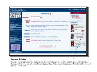
31. Chapter 2 – Data Sources Useful Data Sources: In many instances, you will collect data specific to a specific question of interest through research or survey.

32. Chapter 2 – Survey Research Basic Steps of Survey Research: • Step 1: State the goals of the research • Step 2: Develop the budget (time, money, staff) • Step 3: Create a research design (target population, frame, sample size) • Step 4: Choose a survey type and method of administration • Step 5: Design a data collection instrument (questionnaire) • Step 6: Pretest the survey instrument and revise as needed • Step 7: Administer the survey (follow up if needed) • Step 8: Code the data and analyze it

33. Chapter 2 – Survey Research Survey Types (You should acquaint yourselves with the characteristics of each – Table 2.12). • Mail • Telephone • Interviews • Web • Direct Observation

34. Chapter 2 – Survey Research Survey Guidelines: • Plan– What is the purpose of the survey? Consider staff expertise, needed skills, degree of precision, budget. • Design – Invest time and money in designing the survey. Use books and references to avoid unnecessary errors. • Quality – Take care in preparing a quality survey so that people will take you seriously. • Pilot Test– Pretest on friends or co-workers to make sure the survey is clear. • Buy-in – Improve response rates by stating the purpose of the survey, offering a token of appreciation or paving the way with endorsements. • Expertise – Work with a consultant early on.