Download
1 / 33
340 likes | 472 Views
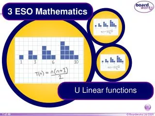
3 ESO Mathematics. U Linear functions. A8 Linear and real-life graphs. Contents. A8.2 Gradients and intercepts. A8.3 Analytical expression. A8.1 Plotting Linear graphs. A8.4 Parallel lines. A8.5 Distance-time graphs. A8.6 Speed-time graphs. Plotting graphs of linear functions. x. –3.

E N D
3 ESO Mathematics U Linear functions
A8 Linear and real-life graphs Contents A8.2 Gradients and intercepts A8.3 Analytical expression A8.1 Plotting Linear graphs A8.4 Parallel lines A8.5 Distance-time graphs A8.6 Speed-time graphs
Plotting graphs of linear functions x –3 –2 –1 0 1 2 3 y = 2x + 5 For example, y to draw a graph of y = 2x + 5: 1) Complete a table of values: y = 2x + 5 –1 1 3 5 7 9 11 2) Plot the points on a coordinate grid. 3) Draw a line through the points. x 4) Label the line. It is very recommendable to add the points of intersection to your table.
Plotting graphs of linear functions You can find the points of intersection very easily. y In the example, y = 2x + 5: • If you make x = 0, you obtain y: • y = 2 · 0 + 5 y = 5 y = 2x + 5 2) If you make y = 0, you obtain x: 0 = 2x + 5 2x = -5 x = -5 / 2 x
A8 Linear and real-life graphs A8.1 Linear graphs Contents A8.3 Analytical expression A8.2 Gradients and intercepts A8.4 Parallel lines A8.5 Distance-time graphs A8.6 Speed-time graphs
Gradients of straight-line graphs y y an upwards slope a horizontal line a downwards slope y x x x The gradient of a line is a measure of how steep the line is. The gradient of a line can be positive, negative or zero if, moving from left to right, we have Positive gradient Zero gradient Negative gradient If a line is vertical its gradient cannot by specified.
Finding the gradient from two given points the gradient = (x2, y2) (x1, y1) change in y change in x x y2 – y1 the gradient = x2 – x1 If we are given any two points (x1, y1) and (x2, y2) on a line we can calculate the gradient of the line as follows, y y2 – y1 Draw a right-angled triangle between the two points on the line as follows, x2 – x1
Calculating gradients • A8.3 Parallel and perpendicular lines • A8.3 Parallel and perpendicular lines
A8 Linear and real-life graphs A8.1 Linear graphs Contents A8.2 Gradients and intercepts A8.3 Analytical expression A8.4 Parallel lines A8.5 Distance-time graphs A8.6 Speed-time graphs
The general equation of a straight line The general equation of a straight line can be written as: y = mx + c The value of m tells us the gradient of the line. The value of c tells us where the line crosses the y-axis. This is called the y-interceptand it has the coordinate (0, c). For example, the line y = 3x + 4 has a gradient of 3 and crosses the y-axis at the point (0, 4).
The gradient and the y-intercept 1 x 2 2 Complete this table: 3 (0, 4) (0, –5) (0, 2) –3 (0, 0) y = x y = –2x – 7 (0, –7)
Rearranging equations into the form y = mx + c The equation of a straight line is 2y + x = 4. Find the gradient and the y-intercept of the line. 2y = –x + 4 1 subtract x from both sides: 2 divide both sides by 2: –x + 4 y = 2 y = – x + 2 Sometimes the equation of a straight line graph is not given in the form y = mx + c. Rearrange the equation by performing the same operations on both sides, 2y + x = 4
Rearranging equations into the form y = mx + c 1 1 y = – x + 2 2 2 – Sometimes the equation of a straight line graph is not given in the form y = mx + c. The equation of a straight line is 2y + x = 4. Find the gradient and the y-intercept of the line. Once the equation is in the form y = mx + c we can determine the value of the gradient and the y-intercept. So the gradient of the line is 2. and the y-intercept is
Substituting values into equations A line with the equation y = mx + 5 passes through the point (3, 11). What is the value of m? To solve this problem we can substitute x = 3 and y = 11 into the equation y = mx + 5. This gives us, 11 = 3m + 5 6 = 3m subtract 5 from both sides: 2 = m divide both sides by 3: m = 2 The equation of the line is therefore y = 2x + 5.
A8 Linear and real-life graphs A8.1 Linear graphs Contents A8.2 Gradients and intercepts A8.3 Analytical expression A8.4 Parallel lines A8.5 Distance-time graphs A8.6 Speed-time graphs
Parallel lines 2y = –6x + 1 subtract 6x from both sides: divide both sides by 2: –6x + 1 y = 2 If two lines have the same gradient they are parallel. Show that the lines 2y + 6x = 1 and y = –3x + 4 are parallel. We can show this by rearranging the first equation so that it is in the formy = mx + c. 2y + 6x = 1 y = –3x + ½ The gradient m is –3 for both lines and so they are parallel.
A8 Linear and real-life graphs A8.1 Linear graphs Contents A8.2 Gradients and intercepts A8.3 Analytical expression A8.5 Distance-time graphs A8.4 Parallel lines A8.6 Speed-time graphs
Formulae relating distance, time and speed DISTANCE distance time = SPEED TIME speed distance speed = time It is important to remember how distance, time and speed are related. Using a formula triangle can help, distance = speed × time
Distance-time graphs 20 distance (miles) 15 10 5 0 0 15 30 45 60 75 90 105 120 time (mins) In a distance-time graph the horizontal axis shows time and the vertical axis shows distance. For example, John takes his car to visit a friend. There are three parts to the journey: John drives at constant speed for 30 minutes until he reaches his friend’s house 20 miles away. He stays at his friend’s house for 45 minutes. He then drives home at a constant speed and arrives 45 minutes later.
Finding speed from distance-time graphs change in distance gradient = change in time distance change in distance change in time time How do we calculate speed? Speed is calculated by dividing distance by time. In a distance-time graph this is given by the gradient of the graph. = speed The steeper the line, the faster the object is moving. A zero gradient means that the object is not moving.
Distance-time graphs change in speed acceleration = time When a distance-time graph is linear the objects involved are moving at a constant speed. Most real-life objects do not always move at constant speed, however. It is more likely that they will speed up and slow down during the journey. Increase in speed over time is called acceleration. It is measured in metres per second per second or m/s2. When speed decreases over time is often is called deceleration.
Distance-time graphs This distance-time graph shows an object accelerating from rest before continuing at a constant speed. distance distance time time This distance-time graph shows an object decelerating from constant speed before coming to rest. Distance-time graphs that show acceleration or deceleration are curved. For example,
A8 Linear and real-life graphs A8.1 Linear graphs Contents A8.2 Gradients and intercepts A8.3 Parallel and perpendicular lines A8.6 Speed-time graphs A8.4 Interpreting real-life graphs A8.5 Distance-time graphs
Speed-time graphs 20 speed (m/s) 15 10 5 0 0 5 10 15 20 25 30 35 40 time (s) Travel graphs can also be used to show change in speed over time. For example, this graph shows a car accelerating steadily from rest to a speed of 20 m/s. It then continues at a constant speed for 15 seconds. The brakes are then applied and it decelerates steadily to a stop. The car is moving in the same direction throughout.
Finding acceleration from speed-time graphs speed change in speed change in speed gradient = change in time change in time time Acceleration is calculated by dividing speed by time. In a speed-time graph this is given by the gradient of the graph. = acceleration The steeper the line, the greater the acceleration. A zero gradient means that the object is moving at a constant speed. A negative gradient means that the object is decelerating.