Download
1 / 11
120 likes | 227 Views
Ch 13 Chemical Equilibrium. Partition Functions K LeChatelier’s Principle K(T), K(p). I. Chemical Equilibrium; K = f(N). Consider gas phase rxn A(g) ↔ B(g) Equilibrium constant = K = N B /N A

E N D
Ch 13 Chemical Equilibrium Partition Functions K LeChatelier’s Principle K(T), K(p)
I. Chemical Equilibrium; K = f(N) • Consider gas phase rxn A(g) ↔ B(g) • Equilibrium constant = K = NB /NA • At constant T and p, G is the thermodynamic function that characterizes equilibrium. dG = -SdT + Vdp + ΣμidNi = ΣμidNi = 0 at equilibrium or μA = μB • Eqn 11.47 defines μ = -kT ℓn (q/N)
K = f(q) • A and B have their own set (ladder) of energy levels beginning at ground state energies ε0A and ε0B, respectively. Fig 13.1 • q’A = partition function = [exp(-ε0Aβ) + exp(ε1Aβ) + exp(ε2Aβ) + …] • μA = -kT ℓn (q’A/N) • qA = reduced partition fnt with ε0A factored out = exp(ε0Aβ) [exp(-ε0Aβ) + exp(-ε1Aβ) + exp(-ε2Aβ) + …] = exp(ε0Aβ) q’A
K = f(q) • K = NB/NA= q’B/q’A = qB/qA exp(- [ε0B - ε0A]β) = qB/qA exp(- Δε0β) Eqn 13.10 • More complex rxn: aA +bB ↔ cC • K = NCc/[NAaNBb] = Eqn 13.18 which shows q and ε0 terms • Ex. 13.2, prob 6
Vibrational Energy Reference Level • If you use bottom of the well = 0 Eqn 11.26 for qvib = exp (-hνβ/2)/[1- exp (-hνβ)]. Then energy from dissociation limit to bottom of well = - ε0 • If you use ZPE as 0 Eqn 13.21 for qvz = exp [1- exp (-hνβ)]-1. Then energy from ZPE to dissociation limit = D or D0 (T11.2)
K=f(p) • K Kp using n = pV/RT or N = pV/kT • Kp = [pCc/[pAa pBc] Eqn 13.29 = (kT)c-a-b [q0Cc/[q0Aa q0Bb] exp(ΔDβ) • q0 = q/V • μ = μ0 + kT ℓn p = std state chem pot and term that depends on p • Ex 13.3, prob 1
II. LeChatelier’s Principle • Given a system at equilibrium at constant T and p, ΔG = 0 and G is at a minimum. Any disturbance on the system will increase G. • The LeChatelier Prin says that the system will return to equilibrium in a way that opposes disturbance. Note that K does not change for all perturbations. Fig 13.4
II.A. K = f(T) • See Thermody. Relationships (p 2) for van’t Hoff Eqn and Gibbs-Helmholtz Eqn. • A(g) ↔ B(g) μA = μB at equilibrium or • μA = μA0 + kT ℓn pA = μB = μB0 + kT ℓn pB • ℓn (pB/pA) = ℓn Kp = -(μB0 - μA0)kT = -∆μ0/kT • ∆μ0 = ∆h0 - T∆s0 (partial molar quant) • ℓn Kp = -∆μ0/kT = [∆h0 - T∆s0]/kT
Van’t Hoff Eqn • ℓn Kp = -∆μ0/kT = - [∆h0 - T∆s0]/kT • Take partial w/respect to T and assume ∆h0 and ∆s0 are independent of T. • δ ℓn Kp /δT = - δ{[∆h0 - T∆s0]/kT}/δT = ∆h0/kT2 Eqn 13.37 • Or δ ℓn Kp /δ(1/T) = - ∆h0/k Eqn 13.38 • Plot ℓn Kp vs 1/T and slope = - ∆h0/k • Ex 13.4, Prob 5
Gibbs-Helmholtz Eqn; G(T) • δ (G/T)/δT = - H(T)/T2 Eqn 13.43; see also p 2 of Thermodynamic Relationships • Recall ∆G = -RT ℓn K
II.B. K = f(p) • (δ ℓn K/δp)T = - ∆v/kT PMV • Ex 13.6