Download
1 / 21
210 likes | 317 Views
Gamma-ray Large Area Space Telescope. The High Energy Gamma-Ray Sky after GLAST Julie McEnery NASA/GSFC. Outline. GLAST/LAT instrument description LAT/GLAST Performance Sensitivity Energy Range Angular resolution Field of view/Duty cycle

E N D
Gamma-ray Large Area Space Telescope The High Energy Gamma-Ray Sky after GLAST Julie McEnery NASA/GSFC
Outline • GLAST/LAT instrument description • LAT/GLAST Performance • Sensitivity • Energy Range • Angular resolution • Field of view/Duty cycle • Slew time – prompt observations of interesting events • Analysis time/notification time – how well do we play with others? Alerts, availability of data? • Science highlights – source counts, what kinds of things might GLAST achieve.
GLAST Overview Two Instruments: Large Area Telescope (LAT) >2.5 sr 20 MeV - 300 GeV GLAST Burst Monitor (GBM) >8 sr 10 keV – 25 MeV Launch: Fall 2007 Lifetime: 5 years (10 year goal) Large Area Telescope (LAT) GLAST Burst Monitor (GBM)
e– e+ Pair Conversion Technique The anti-coincidence shield vetos incoming charged particles. photon converts to an e+e- pair in one of the conversion foils The directions of the charged particles are recorded by particle tracking detectors, the measured tracks point back to the source. The energy is measured in the calorimeter Tracker: angular resolution is determined by: multiple scattering (at low energies) => Many thin layers position resolution (at high energies) => fine pitch detectors Calorimeter: Enough X0 to contain shower, shower leakage correction. Anti-coincidence detector: Must have high efficiency for rejecting charged particles, but not veto gamma-rays
Tracker e– e+ ACD [surrounds 4x4 array of TKR towers] Calorimeter Systems work together to identify and measure the flux of cosmic gamma rays with energy 20 MeV - >300 GeV. Large Area Telescope • Precision Si-strip Tracker (TKR)18 XY tracking planes. 228 m pitch). High efficiency. Good position resolution (ang. resolution at high energy) 12 x 0.03 X0 front end => reduce multiple scattering. 4 x 0.18 X0 back-end => increase sensitivity >1GeV • CsI Calorimeter(CAL) Array of 1536 CsI(Tl) crystals in 8 layers. Hodoscopic => Cosmic ray rejection. => shower leakage correction. 8.5 X0 => Shower max contained <100 GeV • Anticoincidence Detector (ACD) Segmented (89 plastic scintillator tiles) => minimize self veto Height/Width = 0.4 => Large field of view
LAT performance • Angular resolution improves rapidly as a function of energy. • Less dominated by background at higher energies. • Effective area remains flat from 1 GeV up to at least 300 GeV Back Front
Field of View • The LAT is self triggering and has a large aspect ratio, this results in a very large field of view. • The angular resolution also varies as a function of inclination angle, this effect is stronger at lower energies.
Survey Mode • The default operating mode for GLAST will be a survey mode where the LAT is tilted 35 degrees above the orbit plane for one orbit and 35 degrees below for the next. This results in full sky coverage every 2 orbits (i.e. 190 minutes). Sampling pattern over long durations Sampling pattern on short timescales
LAT Sensitivity - I • Sensitivity for 1 year (red) and 5 years (blue) in survey mode (does not include electronic deadtime and SAA passages). • Assumes a source with -2.1 spectrum. • Assume a diffuse background flux of 1.5e-5 phcm-2s-1 • Peak sensitivity is at a few GeV. 5σ/5photons
LAT Sensitivity - II • A single curve does not tell the full story. • The sensitivity is a function of spectral index. • Sensitivity will be a strong function of position with respect to the Galactic plane. • As one moves to higher and higher energies (and shorter timescales) this becomes less true (no longer background dominated)
How many sources - AGN? • AGN estimates range from 1000-10000 • Using the luminosity function described by Chiang and Mukherjee (1998) we estimate that the LAT might detect (in one year): • 2700 > 100 MeV • 1950 > 1GeV • 350 > 10 GeV. • The large number of sources and wide energy range over which they are observed will allow population studies of gamma-ray bright AGN.
Transients - Gamma-ray bursts • Relative to EGRET • Large effective area • Low deadtime ~25 μs (cf 100 ms for EGRET) • Large FoV • Onboard transient search – rapid notification to the community. • How many? • GBM ~ 200/year • LAT, who knows? Depends on their behaviour at GeV energies. But we can make a educated guess. • Phenomological model to generate a sample GRB consistent with BATSE observations and extrapolate high energy spectrum and temporal behaviour, and apply EBL attenuation based on the best fit model from Kneiske et al 2004. E 30 MeV 100MeV 1GeV 5 GeV 10 GeV # GRB (10 ph>E) 52 45 20 8 4
Pulsars • From studies of LogN/LogS distributions and spin down energy, we might expect to see ~100s of pulsars, we will likely not be able to identify all of these as pulsars. • Distinguish between models by studying the ratio of radio-loud to radio quiet pulsars.
AGN variability It is not just how many we see, but what we can do with them that counts! • The LAT will provide long, evenly sampled lightcurves, allowing us to characterise the variability over a wide range of timescales. • Contribute to our understanding of the underlying causes of the variability • LAT can search for QPOs on timescales of weeks to months and possible periodic signals (due to e.g. binary black holes). These signals would appear as a spike/peak on the plot of the PSD.
AGN Variability • To study emission mechanisms it is useful to be able to resolve individual flares. • Short timescale variability will also be seen but is more likely to be at the lower energy end of the LAT range (sensitivity > 1 GeV is still photon limited after a weeks observation). • With the wide FoV and scanning, the LAT will be sensitive to catching rare, but strong events. EGRET observations (red points) of a flare from PKS 1622-297 in 1995 (Mattox et al), the black line is a lightcurve consistent with the EGRET observations and the blue points are simulated LAT observations.
Spectral Studies • The improved sensitivity and energy resolution at high energies will allow the LAT to measure spectral breaks for many sources Simulation of 6 months of data from 1ES 0836+710 (z=2.2), average flux is consistent with the EGRET observations, but the flux and spectral index are variable. Use the best fit model from Kneiske et al to simulate attenuation on the EBL. LAT simulation of the Vela pulsar illustrating the difference between the polar cap and outer gap models. But there will be many sources where we cannot…
Transients – operational issues • Both the LAT and the GRB perform onboard searches for GRB. • On detection of a GRB the spacecraft can autonomously repoint to keep the GRB location within the LAT FoV. • Rate of ~1/week for GRB which trigger within the LAT FoV. • 1/months for GRB outside the LAT FoV. • Ensures a fairly large sample of GRB with GeV observations of the prompt and early afterglow phases. • Both the LAT and GRB positions from onboard analysis will be rapidly communicated via GCN (requirement is 7 s from spacecraft to GCN). • Refined analysis/position on GBM (and possibly a subset of the LAT) data will be available 10min – 1 hour later. • Full LAT ground analysis ~12-24 hours later.
GRB Afterglows Improved sensitivity allows us to see new classes of variable sources such as GRB afterglows. Models of the afterglow emission by Sari and Esin (1999) predict that the luminosity of the GRB afterglow at GeV energies will be comparable to that at X-ray energies. GLAST may observe a GeV afterglow for several hours after the burst.
Spatial resolution Likely to be something like dozens of positional coincidences with SNR, a few will be spatially resolved. • For some SNR candidates, the LAT sensitivity and resolution will allow mapping to separate extended emission from the SNR from possible pulsar components. • Energy spectra for the two emission components may also differ. • Resolved images will allow observations at other wavelengths to concentrate on promising directions. (a) Observed (EGRET) and (b) simulated LAT (1-yr sky survey) intensity in the vicinity of γ-Cygni for energies >1 GeV. The dashed circle indicates the radio position of the shell and the asterisk the pulsar candidate proposed by Brazier et al. (1996).
LAT Legacy • Sensitive survey of the sky from 30 MeV to >300 GeV • Thousands of high energy gamma-ray sources. • Many more detections of objects from known source classes. • Likely to discover new classes of high energy gamma-ray emitters. • Many will be unidentified. • Many SNRs and galaxy clusters will be unresolved or coarsely mapped by the LAT. • Resolving the unresolved sources will help identify the LAT sources. • Mapping the gamma-ray emission from extended sources is likely to be very scientifically rewarding. • Efficient observing mode, improved sensitivity and increased effective area combine to provide superb monitoring of the entire GeV sky on timescales of hours to years.