Download
1 / 24
240 likes | 381 Views
NEMO Users meeting, Daget and Weaver, 2006/06/09. Estimating background-error covariance parameters in a variational ocean data assimilation system through the use of ensemble-based methods. OPAVAR / NEMOVAR Introduction. 2 . Objectives.

E N D
NEMO Users meeting, Daget and Weaver, 2006/06/09 Estimating background-error covariance parameters in a variational ocean data assimilation system through the use of ensemble-based methods
OPAVAR / NEMOVAR Introduction 2. Objectives To develop a global ocean variational assimilation system for OPA for diverse applications Current applications: • Initialization for climate forecasting (seasonal and beyond) with coupled models • European projects ENACT (2001-2004) and ENSEMBLES (2004-2008) • Ongoing collaboration with ECMWF for future operational implementation • Global ocean reanalysis (multi-annual/-decadal) • ENACT • CLIVAR Future applications: • Initialization for ocean forecasting (days to weeks) • MERCATOR
OPAVAR / NEMOVAR introduction 3. General formulation Minimize where background term observation term subject to the constraint We construct the control vector so that • Improves the conditioning of the minimization • Allows for nonlinear balance and smoothness constraints (they are embedded in )
OPAVAR / NEMOVAR Introduction 4. The linearized transformation G Univariate smoothing Rescaling Linear multivariate balance Linear ocean model integration Interpolation 3D-Var (FGAT) 4D-Var
OPAVAR / NEMOVAR introduction 5. The balance operator K Kxy represents the transformation from the variable y into x The variables with a subscript B/U represent the balanced/unbalanced components of the variables
OPAVAR/NEMOVAR introduction 6. Scaling factors D The scaling factors in D are chosen to approximate the standard deviations of the background error of the variable in
OPAVAR/NEMOVAR introduction 7. Univariate smoothing F Χ is a scalar field, which in the current context would correspond to one of the variables of the control vector v Kp is a metric (diffusion) tensor Univariate smoothing is performed in grid-point space and is achieved through successive applications of a generalized diffusion operator. The product of a linearized generalized diffusion operator with its transpose corresponds to the correlation operator use for representing background errors
Estimating background-error covariance 8. Intoduction xai+1 xai xbi+1 xbi i i+1 3DVAR with IAU xbi = xai
Estimating background-error covariance 9. Introduction i-1 i-1 i i i+1 i+1 i+2 i+2 i+3 i+3 i+4 i+4 3DVAR with IAU Ref xib,Ref - = δxb,M1 M1 xib,M1
Estimating background-error covariance 10. Theory If we use 2 different perturbed analysis, we have :
Estimating background-error covariance 11. Windstress perturbations Different windstress perturbations (1993-01-01) -0,1 0,1 -0,1 0,1 -0,1 0,1 -0,1 0,1 Daily windstress : calculated from the difference between different wind stress data sets (ERA-40 and CORE) prepared at ECMWF
Estimating background-error covariance 12. SST perturbations Different SST perturbations (1993-01-01) -1 1 -1 1 -1 1 -1 1 Daily SST : calculated from the difference between different SST analyses (Reynolds 2Dvar and Reynolds Olv2 or ERSSTv2 and HadlSST1.1) prepared at ECMWF.
Estimating background-error covariance 13. SST Perturbations SST perturbations hoevmollers (latitude = 56S) Without correlation 7 days correlation 1994 T : time correlation factor 0 years years 1993 1993 360 360 longitude longitude SST is spatially correlated, but not temporally correlated. SST is temporally correlated using 2 passes of a recursive filter, which is equivalent to applying the smoothing function (SOAR).
Estimating background-error covariance 14. Observations perturbations Observations : obtained as random realizations of the Gaussian probability distribution function whose mean is zero, and whose covariance matrix corresponds to the specified observation error covariance matrix R :
Estimating background-error covariance 15. Ensemble Compute the unbalanced components of the differences Obs01 Obs02 Obs03 Obs04 Obs05 Obs06 Obs07 Obs08 Obs09 Obs10 Obs11 Obs12 Obs13 Obs14 Obs15 Obs16 SST1, Windstress 1 SST2, Windstress 2 SST3, Windstress 3 SST4, Windstress 4 SST0, Windstress 0, Obs00
Estimating background-error covariance 16. Softwares used Prepifs : create experiment xcdp : manage experiment
Estimating background-error covariance 17. Temperature standard deviation Default parameterization 50 m Ensemble computation 50 m
Estimating background-error covariance 18. Temperature standard deviation Default parameterization 100 m Ensemble computation 100 m
Estimating background-error covariance 19. Unbalanced salinity standard dev. Default parameterization 50 m Ensemble computation 50 m
Estimating background-error covariance 20. Unbalanced salinity standard dev. Default parameterization 100 m Ensemble computation 100 m
Estimating background-error covariance 21. Unbalanced SSH standard dev. Default parameterization Ensemble computation
Estimating background-error covariance 22. Use standard deviation computed M1 i-1 i i+1 i+2 i+3 i+4 Compute new standard deviation The variance computed with ensemble method is used to modify the diagonal of the background-error covariance matrix each cycle.
Estimating background-error covariance 23. Conclusions and perspectives The variance computed with ensemble method is strongly different than the parameterized variance, especially for unbalanced salinity and unbalanced SSH. A new experiment using variance computed with ensemble method is designed, is running and will be tested. The covariance will be computed. New operators, which permit to use covariance, will be added
References L. Berre, S. E. Stefanescu and M. B. Pereira, 2006: The representation of the analysis effect in three error simulation techniques. Tellus A, 58:196. N. Daget, 2006: Utilisation d’un filtre récursif 1D pour corréler les perturbations de la SST. Technical Report TR/CMGC/06/17, CERFACS. Hayden, C. M., and R. J. Purser, 1995: Recursive filter objective analysis of meteorological fields : application to NESDIS operational processing. J. Appl. Meteor., 34, 3-15. Lorenc, A. C., 1992: Iterative analysis using covariance functions and filters. Q.uart J. Roy. Meteor. Soc., 118, 569-591. Purser, R. J., 2002: Numerical aspect of t he application of recursive filters to variational statistical analysis. Part I: spatially homogeneous and isotropic gaussian covariances. Mon. Wea. Rev., 131, 1524-1535 S. Ricci, 2005: A. T. Weaver, J. Vialard and P. Rogel. Incorporating state-dependent temperature-salinity constraints in the background-error covariance of variational ocean data assimilation. Monthly Weather Review, 133: 317-338. J. Vialard, A. T. Weaver, D. L. T. Anderson and P. Delecluse, 2003: Three- and four-dimensional variational assimilation with an ocean general circulation model of the tropical Pacific Ocean. Part 2: physical validation. Monthly Weather Review, 131: 1379-1395. A. T. Weaver, C. Deltel, E. Machu, S. Ricci and N. Daget, 2006: A multivariate balance operator for variational ocean data assimilation. Q. J. Roy. Meteor. Soc., In press. A. T. Weaver, J. Vialard and D. L. T. Anderson, 2003: Three- and four-dimensional variational assimilation with an ocean general circulation model of the tropical Pacific Ocean. Part 1: formulation, internal diagnostics and consistency checks. Monthly Weather Review, 131: 1360-1378. A. T. Weaver and P. Courtier, 2001: Correlation modeling on the sphere using a generalized diffusion equation. Quaterly Journal of the Royal Meteorological Society, 127:1815-1846. A. Weisheimer, 2005: SST and windstress perturbations for seasonal and annual simulations. ENSEMBLES RT1 documentation, ECMWF.