Download
1 / 62
660 likes | 872 Views
Violations of the fluctuation dissipation theorem in non-equilibrium systems. Introduction:. glassy systems: very slow relaxation. quench from high to low temperature: equilibrium is reached only after very long times. physical aging. out-of equilibrium dynamics: energy depends on time

E N D
Violations of the fluctuation dissipation theorem in non-equilibrium systems
Introduction: glassy systems: very slow relaxation quench from high to low temperature: equilibrium is reached only after very long times physical aging • out-of equilibrium dynamics: • energy depends on time • response and correlation depend on 2 times (aging not restricted to glassy systems)
aging-experiment: quench Thigh Tlow <Tg measure some dynamical quantity related to the -relaxation physical aging: glassforming liquids:
quench: measurement of different quantities: measurement: one-time quantities: energy, volume, enthalpy etc. equilibrium: t-independent t=0 t=tw time two-time quantities: correlation functions equilibrium: Y depends on time-difference t-tw : ensemble average typical protocol:
quench: sudden change of temperature from Thigh to Tlow qualitative features are often independent of the cooling rate experiment: simulations: theory: initial temperature: experiment: > Tg simulation: 'high' theory: 'high' meaning of quench:
experimental results – one-time quantities: polystyrene , Tg=94.8oC volume recovery (Simon, Sobieski, Plazek 2001) quench from 104oC data well reproduced by TNM model
TNM model (used quite frequently in the analysis): Y=enthalpy, volume, etc. (tw=0) Tool-Narayanaswamy-Moynihan (TNM): : fictive temperature x: nonlinearity parameter (=const.)
experimental results – dielectric response: dielectric relaxation of various glassforming liquids: Leheny, Nagel 1998 Lunkenheimer, Wehn, Schneider, Loidl, 2005 Tg=185K '' but '' re-equilibration is always determined by the -relaxation (independent of frequency)
T=0.4 Cst usually not observable in lab glasses simulation results – two-time quantities: binary Lennard-Jones liquid Kob, Barrat 2000 Tc=0.435 quench T>Tc T<Tc
t1 t3 t2 t4 model calculations: domain-growth e.g. 2d Ising-model self similar structures but no equilibrium
plateau value: C0 T=0.5 ) w ,t t + w C(t t w 1.0 0.8 short times: stationary dynamics within domains 0.6 t / s long times: domainwall motion 0.4 0.2 0.0 -2 -1 0 1 2 3 4 5 10 10 10 10 10 10 10 10 ferromagnet:
main messages: • typical aging experiment: • quench from some Thigh to Tlow • after tw: measurement • frequent observations: • relaxation time increases with tw • equilibrium is reached for (extremely) long tw • glasses: re-equilibration is determined • by -relaxation • models: two-step decay of C(t,tw) some debate about t-tw superposition and other details
H0 H=0 violations of the FDT: dynamic quantity: correlation: response: apply a small field H linear response
: FDT – equilibrium: stationarity: impulse response equilibrium statistical mechanics: FDT:
FD-plot: slope: 1/T C equilibrium – integrated response: (step response function):
T='high' T(working) FDT violation: (fluctuation-dissipation ratio) non-equilibrium: quench at t=0 start of measurement: tw fluctuation-dissipation relation FDR: (definition of X)
integrated response: equilibrium: fluctuation-dissipation ratio: some models in the scaling regime:
SK model (RSB) p-spin model (1RSB) spherical model, Ising model FD-plots: examples:
short times: FDT: X=1 long times: X<1 typical behavior of the FDR:
effective temperature Teff: definition of an effective temperature: (there are other ways to define Teff) examples: coarsening models: p-spin models (1-RSB): (~MCT – glassy dynamics)
FDR – experimental examples: Supercooled liquid dielectric Polarization noise Grigera, Israeloff, 1999 spinglas SQUID-measurement of magnetic fluctuations Herisson, Ocio 2002 glycerol, T=179.8 K (Tg=196 K) CdCr1.7In0.3S4, T=13.3 K (Tg=16.2 K)
FDR – example from simulations: binary Lennard-Jones system Kob, Barrat 2000
consider a dynamical variable M(t) coupled linearly to a thermometer with variable x(t) linear coupling: net power gain of the thermometer: linear response theory calculation of : thermometer: correlation response Teff is a temperature - theory (Cugliandolo et al. 1997)
dynamic quantities a0: a=0: calculation of Teff - cont:
first term: fast thermometer – Rx decays fast second term: tt' , thermometer in equilibrium at Tx: -tCx=TxRx calculation of Teff – still cont:
calculation of Teff – result: • 'protocol': • connect thermometer to a heat bath at Tx • disconnect from heat bath and connect to the glas • if the heat flow vanishes: • Teff=Tx
fluctuation-dissipation relations – theoretical models: slow dynamics: solution of Newtonian dynamics impossible on relevant time scales standard procedures: consider stochastic models: Langevin equations (Fokker-Planck equations) master equations
consider some statistical mechanical model (very often spin models) dynamical variables si, i=1,...,N Hamiltonian H Langevin equation: stochastic force deterministic force stochastic force: 'gaussian kicks' of the heat bath Langevin equations:
Langevin equation for variable x(t): causality: x cannot depend on the noise to a later time correlation function: time-derivatives: Langevin equations – FDR
without proof: definition of the asymmetry: FDR: Langevin equations – FDR – cont.
time reversal symmetry: stationarity: FDT: Langevin equations – FDR – equilibrium
Langevin equation for diffusion: diffusion in a potential: solution: (inhomogeneous differential equation) decay of initial condition x(0)=x0 inhomogeneity FDR – Ornstein-Uhlenbeck process: diffusion in a harmonic potential: Ornstein-Uhlenbeck
correlation function: response: asymmetry: FD ratio: OU-process excercise: calculate
decay of initial state equilibrium correlation equilibrium: equilibrium is reached for s due to the decay OU-process cf - cont:
asymmetry: OU-process: OU-process FDR:
independent of t equilibrium is reached after long times OU-process FDR cont:
spins on a lattice: Ising: spherical: global constraint S-FM: exact solution for arbitrary d another example: spherical ferromagnet
stochastic dynamics: Langevin equations: stochastic forces: Gaussian Lagrange multiplier z(t)=2d+(t) solution of the L-equations: Fourier-transform all dynamical quantities
response: stationary regime: aging regime: correlation and response (T<Tc): correlation function: d=3: Tc=3.9568J/k stationary regime: short times aging regime: short times
T=0.5 ) w ,t t + w C(t t w 1.0 0.8 short times: stationary dynamics within domains long times: domainwall motion 0.6 t / s 0.4 0.2 quasi-equilibrium at Tc 0.0 coarsening: domains grow and shrink -2 -1 0 1 2 3 4 5 10 10 10 10 10 10 10 10 correlation function:
stationary regime: FDT at Tc aging regime: limiting value: domain walls are in disordered state typical for coarsening systems fluctuation dissipation ratio (T<Tc):
(free) energy order parameter population of ‘states‘ (configurations): dynamics: transitions FDR for master equations: stochastic evolution in an energy landscape
master equation: loss gain detailed balance: transition rates: example: Metropolis: FDR for master equations - cont:
W0 W0 xk-1 xk+1 xk for nearest neighbor transitions solution: Fourier transform gaussian master equations - example: 1 dim. random walk:
preparation in initial states: T= T(working) e.g. quench: time evolution at T: propagator: same master equation as for populations
calculation of dynamical quantities: correlation function: response: coupling to an external field H ?
perturbed transition rates: equilibrium: (not sufficient to fix the transition rates) choice: (Ritort 2003) detailed balance: typically ==1/2
asymmetry is not related to measurable quantities: response: perturbation theory FDR for Markov processes 'asymmetry' looks similar to the FDR for Langevin equations