Download
1 / 27
270 likes | 422 Views
New approaches in extreme-value modeling. A.Zempl éni, A. Beke, V. Csisz ár (Eötvös Loránd University, Budapest) Flood Risk Workshop, 08.07.2002. Analysis of extreme values.

E N D
New approaches in extreme-value modeling A.Zempléni, A. Beke, V. Csiszár (Eötvös Loránd University, Budapest) Flood Risk Workshop, 08.07.2002
Analysis of extreme values • Probably the most important part of the project (its aim: to estimate return levels – values which are supposed to be observed once in a given period, 100 years for example). • Classical methods: based on annual maxima (other values are not used). • Peaks-over-threshold methods: utilize all values higher than a given (high) threshold.
Extreme-value distributions (for modeling annual maxima) Let be independent, identically distributed random variables. If we can find norming constants an, bn such that has a nondegenerate limit, then this limit is necessarily a max-stable or so-called extreme value distribution. X1, X2,…,Xn [max(X1, X2,…, Xn)-an]/ bn
Characterisation of extreme-value distributions • Limit distributions of normalised maxima: Frechet: (x>0) is a positive parameter. Weibull: (x<0) Gumbel: (Location and scale parameters can be incorporated.)
Estimation methods • Maximum likelihood, based on the unified parametrisation: • if • the most widely used, with optimal asymptotic properties, if ξ>-0.5 • Probability-weighted moments (PWM) • Method of L-moments
Probability-weighted moments • Analogous to the method of moments • It puts more weight to the high values • The estimators are got by equating the empirical and the theoretical weighted moments and solving the equations for the parameter vector.
Method of L-moments • The basic characteristics (mean, variance, skewness and kurtosis) of the observed distribution are equated to their respective theoretical values. • These values can be estimated by the help of the probability weighted moments.
Comparison • Maximum likelihood is preferable, since • asymptotic properties are known, allowing the construction of confidence intervals • covariates can be incorporated into the model • For the other methods, there is no firm theory.
Further investigations • Estimates for return levels • Confidence bounds should be calculated, possible methods • based on asymptotic properties of maximum likelihood estimator • profile likelihood • resampling methods (bootstrap, jackknife) • Bayesian approach
Confidence intervals • For maximum likelihood: • By asymptotic normality of the estimator: where is the (i,i)th element of the inverse of the information matrix • By profile likelihood • For other nonparametric methods by bootstrap.
Profile likelihood • One coordinate of the parameter vector is fixed, the maximization is with respect the other components: • Its main advantages: • The uncertainty can be visualized • More exact (asymmetric) confidence bounds • Model selection for nested models is possible by the likelihood ratio test
Model diagnostics • Probability plot (P-P plot), the points: • Quantile plot (Q-Q plot), the points: Both diagram should be close to the unit diagonal if the fit is good.
An example: a simulated 100-element sample of unit exponentials
Peaks over threshold methods • Those events are considered extreme, which exceed a given (high) threshold • Advantages: • More data can be used • Estimators are not affected by the small “floods” • Disadvantages: • Dependence on threshold choice • Declustering not always obvious
Theoretical foundations Let X1, X2,…,Xn be independent, identically distributed random variables. If the normalised maximum of this sequence converges to an extreme value distribution (with parameters μ,σ,ξ), then if y>0 and where The asymptotics holds if n and u increases.
Inference • Similar to the annual maxima method: • Maximum likelihood is to be preferred • Confidence bounds can be based on profile likelihood • Model fit can be analyzed by P-P plots and Q-Q plots • Return levels/upper bounds can be estimated
Threshold selection Mean excess plot: For any u (threshold), plot the mean of X-u (for those observations for which X>u) against u. If the Pareto model is true, this plot should be nearly linear. The interpretation is made difficult by the great variability near the upper endpoint of the observations.
Another, very recent method: maximum cross-entropy • Kullback introduced the concept of probabilistic distance (cross-entropy) of a posterior distribution h(t) from a prior f(t): • The method (Pandey, 2002)minimizes the cross-entropy of x(t) (the observed quantile function of exceedances) with respect to its prior estimate y(t), which is chosen as the exponential (motivated by its central role within the GPD family).
Moment conditions PWM constraints: (usually N=3 is used), where is unbiased estimator for the kth PWM, based on the ordered sample of size n
Some results for Vásárosnamény • Six threshold values were used: 440, 480, 520, 560, 600 and 640 centimetres. • As constraints, we considered the first four PMWs, that is, N=3. • The estimated 100-, 500-, and 1000-year return levels
Comments • The results were not as stable as it was claimed in the original paper. • We intended to add bootstrap confidence bounds to the estimates, but this was too time consuming in its original version and the used simplifications have not proven to be realistic.
Stationary sequences • If the independence does not hold (as it is the case for the original daily observations), the limit of the normalized maxima is still a GEV distribution, if the dependence among far away observations tend to diminish. (See the talk of S. Gáspár.) So the GEV model for annual maxima has sound theoretical background. • For POT models, the maximum of the clusters of exceedances may be used. (Clusters need to be defined).
To cope with nonstationarity • Linear regression-type models can be incorporated into the maximum likelihood framework • Profile likelihood, likelihood-ratio tests can be performed for nested models
Water-level data example: Vásárosnamény • At least two observations per day for each station (there are approx. 50 of them) for 100 years. • Reduction: one observation per day.