Download
1 / 13
130 likes | 242 Views
This study explores the use of kinematical fit to improve resolution in identifying K decay vertex positions and tracking momentums, aiming to enhance vertex efficiency. The fit strategy involves 11 input parameters and 4 constraints, leading to improved separation and potential momentum resolution. The procedure defines delta and employs different Gaussian components to enhance resolution on vertex position and Kaon momentum. Efforts are underway to optimize son momentum tracking efficiency. The project is focused on enhancing efficiency through K decay and son momentum analyses.

E N D
Determination of K vertex efficiency using a kinematical fit F. Ambrosino, P. de Simone, P. Massarotti, V. Patera • Why a kinematical fit • Fit performances: resolutions • K decay vertex efficiencies K charged meeting - 27 april 2004 P. Massarotti
Motivations for a kinematical fit The main aim is to improve the resolution of the neutral vertex position and the secondary charged track momentum (before actually seeing it !!), in order to have detailed vertex efficiencies plots. Other byproducts: • Improve 2 body/3 body separation • Possibly improve K momentum resolution • Improve photons timing resolution
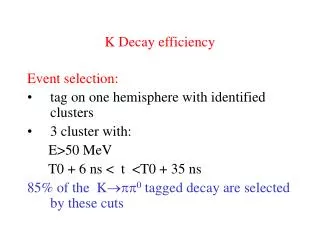
Fit strategy 11 input parameters: • E, x, y, z, t for 2 photon candidates • Delta (see next slide) 4 constraints: • abs( t - | xclu - xv |/c - TOFK) = t0 (2) • Mgg = Mp0 • Angle between K and p0 vs p0 energy from 2 body decay
Fit procedure : definition of delta L.H. L.H. L.H. F.H. F.H. F.H. Vertex Len K Len track = len K – len track
second gaussian sx sy 1.5 cm sz 1. cm third gaussian sx sy 9.5 cm sz 5.5 cm first gaussian sx sy sz 3.5 mm Resolution on vertex position Xrec - Xmc (cm)
second gaussian spx spy 3. MeV/c spz 4. MeV/c first gaussian spx spy spz 1.5 MeV/c third gaussian spx spy 15.5 MeV/c Resolution on Kaon momentum Pxrec - Pxmc (MeV/c)
first gaussian spx spy spz 2.5 MeV/c second gaussian spx spy spz 7. MeV/c third gaussian spx spy spz 25.5 MeV/c Resolution on son momentum Pxrec - Pxmc (MeV/c)
e vertex e vertex Vertex efficiency as a function of K decay length L kaon (cm) L kaon (cm)
e vertex e vertex Vertex efficiency as a function of son momentum Pmod (MeV/c) Pmod (MeV/c) • Kfit selection
•Looking for a neutral vertex using son track •Looking for a neutral vertex using K tag Informations Kaon tracking efficiency Ep,xp,tp Eg,tg,xg p± xK pK lK Kmn tag tm t0 pK p0 Eg,tg,xg
e tracking e tracking tracking efficiency as a function of K decay length L kaon (cm) L kaon (cm)
e tracking e tracking Using the ‘or’ condition : L kaon (cm) L kaon (cm)
e decay Decay efficiency using K tag informations Working on progress L kaon (cm)


![The Determination of K eq for [FeSCN 2+ ]](https://cdn5.slideserve.com/9445046/the-determination-of-k-eq-for-fescn-2-dt.jpg)