Download
1 / 35
350 likes | 473 Views
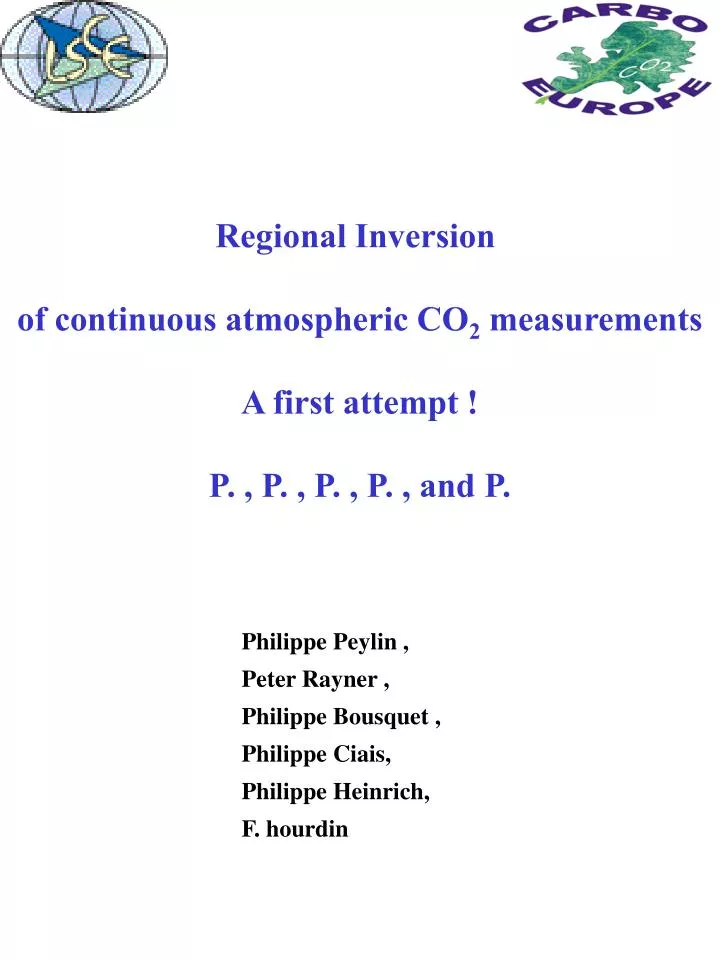
Regional Inversion of continuous atmospheric CO 2 measurements A first attempt ! P. , P. , P. , P. , and P. Philippe Peylin , Peter Rayner , Philippe Bousquet , Philippe Ciais, Philippe Heinrich, F. hourdin. Outline. Measurements over Europes Requirements for regional inversions

E N D
Regional Inversion of continuous atmospheric CO2 measurements A first attempt ! P. , P. , P. , P. , and P. Philippe Peylin , Peter Rayner , Philippe Bousquet , Philippe Ciais, Philippe Heinrich, F. hourdin
Outline • Measurements over Europes • Requirements for regional inversions • Time resolution in an inversion ? • LMDz transport model : - direct approach • - retro-plume approach • European set up : primarily results
The European observing system : Flasks In-situ Aircraft Aircraft (project) AEROCARB database : http://www.aerocarb.cnrs-gif.fr/database.html
Aircraft measurements - Orleans, France CO2 concentrations for all flights PBL Free troposphere
Continuous measurements At Mace Head How to use such information ?
How to assimilate continental sites ? • Transport models are to be improved :- Higher resolution in time and space - Parameterization of PBL • Mesoscale models : boundary problems ! • Nested models : computing time ! • Global with zoom : LMDz model • Data selection in models : - position in space and time properly represented • Prior land fluxes should be improved : - Fossil fuel - Diurnal cycle of biospheric fluxes • Inverse procedure need to be updated :- Spatial resolution of fluxes : pixel ? - Time resolution : identical for fluxes / obs ?
Diurnal rectification effect : Selection of model output according to flask data timing (TM3) Concentrations (ppm) Monthly mean 24 hr Monthly mean Flask timing
[ ppm ] CO2 - fossils [ ppm ] Data selection Spatial position of Schauinsland station in mesoscale model REMO REMO 30m REMO 130m Observations DAYS (Chevillard, 2001)
Spatial resolution of fluxes ? Few large regions All pixels • Aggregation error • Estimation error A 2GtC/yr Sink over Europe, consistent with all Observations (kaminsky et al.) Compromise needed OR all pixel + correlations
Time discretisation Question : Should we average data at the time-resolution of the fluxes we solve for ? - Annual flux : Monthly data ? - Monthly flux : Daily data ? - Satellite : assimilate individual shot ? Little derivation : • Estimation of flux X ={xi, i=1,n} with a temporal distribution xi • Observations Y = {yi, i =1, m} with same errors R • None Bayesien with error
Averaged data Y All data {yi, i =1, m} Same weight for all data Data weight proportional to Hi Hi = Transport o Flux-distribution {xi} High values of Hi correspond to “ low mixing by transport ” and / or “Peak of the flux time-distribution”
Error estimates We can show Uncertainties are always smaller with all individual data
Annual response function sampled each month Time pattern : total respiration (SiB2) Pulse of 1GtC / year Temperate N. Amer. (3rd yr) 25 20 15 Concentration (ppmv) 10 5 month
Monthly response function sampled each day Time pattern : flat Pulse of 1GtC / month Western Europe (July pulse) 40 30 20 Concentration (ppmv) 10 0 -10 Days
Summary of time discretisation ? • Need some caution when using data at higher time resolution than that of the fluxes • Individual terms Hi need to be compared ! • Annual flux / Monthly data is not adapted • Monthly flux / daily data ?? • Solution is probably : solve fluxes at the resolution of the data + time-correlation(equivalent to the “spatial aggregation problem”)
LMDz transport model • GCM from the LMD laboratory (Paris) • Nudged with ECMWF • Global with possible zoom - 0.5 x 0.5 degree in zoom - 4 x 4 degree at the lowest • 19 vertical levels • Backward mode possible grid zoomed over Europe
Inverse Transport : “retro-plume” approach Frederic Hourdin Direct approach : J: measure = mean CO2 per kg of air C: concentration of CO2 (kg / kg air) r: density of air m : distribution of the measure W, t : spatial and temporal domain C is govern by : With - surface flux : s = - C = Ci at t0
Inverse approach : Rewrite measure using the advection/diffusion equation like in lagrange multipliers c*: distribution to be determined Using : • integration by parts • c* that satisfy • 0 = We obtain : Contribution from Initial conditions Flux contribution
Retro-plume approach • Simply run transport backward in time • (need to save all mass flux in a forward run) • C* is the sensitivity to both • surface fluxes / initial conditions • in ppmv / kgC Direct mode / Inverse mode Sample c* according to s distribution Emission according To selected data Source s variable Selection of data J
Example of retro-plumes Schauinsland station in November 1998 Day 1 Day 2 Day 4 Day 8
Mace Head retro-plume Day 4 Day 4 longitude
European Inversion, using continuous data, with high temporal/spatial flux resolution, for a short period (campaign) Only a first attempt !
methodological experiment • Data : 2 sites Mace Head / Schauinsland • Daily average values • Period : Campaign type experiment • one month : November 1998 • Regions : • - Pixels for Western Europe • - Rest of the world with large regions (18) • Time resolution of fluxes : • - Daily for pixels • - monthly for the other large regions • Priors • Pixels Large regions • Flux: Bousquet et al. Bousquet et al. • Error: 100 % of mean 1GtC+correlations (0.8) • Special treatment for initial conditions
Map of regions + 2 sites Mace Head Schauinsland November November
Treatment of initial conditions • Add additional unknowns corresponding to initial conditions • Reduce the size of initial condition problem by projecting on main directions in the data space using SVD. Cinit = H x Pprior (60 x 50000) (50000) (SVD decomposition) U . W . VT x Pprior H’ x P’ (60 x 60) (60) Solve for P’ with : - prior value from global simulation (using bousquet et al. fluxes) - error corresponding to 3 ppm
Model components : MHD 8 Europe Pixels -4 8 Other big regions ppmv -4 8 Initial conditions posterior prior -4 days
Model components : SCH 8 Europe Pixels -4 8 Other big regions ppmv -4 8 Initial conditions posterior prior -4 days
Summary • Regional CO2 flux estimates require complete and permanent monitoring of CO2 • Transport models have to be improved over the continents ! • Selection of the data (time and space) is crucial • Inverse scheme : - High spatial resolution with correlations - Temporal resolution of fluxes adapted to the resolution of the data • Initial conditions seem to be important for campaign based inversions (10 day !) • => Need for other constraints : O2/N2, C14, C13, O18, Radon, …
AEROCARB project: European Inversion - 5 models - European domain for regional models - Boundary from global model (TM3) - Use continuous data over Euro-Siberia (12 sites) - Account for “diurnal rectifier” / selection (during aircraft profiles) • Monthly inversion first • Daily inversion in a second step
Monthly response function sampled each day Time pattern : flat Pulse of 1GtC / month Western Europe (January pulse) Concentration (ppmv) Days
Annual response function sampled each month Time pattern : total respiration (SiB2) Pulse of 1GtC / year Boreal N. Amer. (3rd yr) Concentration (ppmv) month
Conclusions • Regional CO2 flux estimates require a complete and permanent monitoring of “regional” air using atmospheric data (flask & continuous sites, towers, airplane, …) ---> Monitoring of air is essential to estimate European carbon budget. • Currently data limited inversions are becoming model limited inversion as we intend to assimilate continental measurements ----> Transport models have to be improved over the continents. • There is only one carbon cycle. There is no reason to assimilate only atmospheric data. ----> A global carbon assimilation system should be developed Addressing these issues should allow to provide Kyoto relevant estimates of European carbon budget within the next decade.