Download
1 / 14
140 likes | 245 Views
Use of 4 km, 1 hr, Precipitation Forecasts to Drive a Statistical-Distributed Hydrologic Model for Flash Flood Prediction J8.4 20 th Conference on Hydrology, AMS Annual Meeting 2006 Seann Reed 1 , Richard Fulton 1 , Ziya Zhang 1,2 , Shucai Guan 1,3 Presented by John Schaake 4

E N D
Use of 4 km, 1 hr, Precipitation Forecasts to Drive a Statistical-Distributed Hydrologic Model for Flash Flood Prediction J8.4 20th Conference on Hydrology, AMS Annual Meeting 2006 Seann Reed1, Richard Fulton1, Ziya Zhang1,2, Shucai Guan1,3 Presented by John Schaake4 1Hydrology Laboratory, Office of Hydrologic Development National Weather Service, NOAA, Silver Spring, Maryland 2University Corporation for Atmospheric Research 3RS Information Systems, Inc. 4Consultant to Office of Hydrologic Development, Annapolis, MD
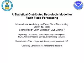
A Statistical-Distributed Model for Flash Flood Forecasting at Ungauged Locations Real-time QPE/QPF simulated historical peaks (Qsp) Archived QPE Initial hydro model states Real-time Historical • The statistical-distributed model outputs gridded flood frequency forecasts. • Here we express flood frequencies in terms of the return period (T) associated with the annual maximum flood.T = 1/p where p is the probability of occurrence in a given year (e.g. If p = 0.5, T = 2 years). Distributed hydrologic model (HL-RDHM) Distributed hydrologic model (HL-RDHM) Max forecasted peaks Statistical Post-processor Simulated peaks distribution (Qsp) (unique for each cell) Forecasted frequencies
Why a frequency-based approach? • Frequency grids provide a well-understood historical context for characterizing flood severity; values relate to engineering design criteria for culverts, detention ponds, etc. • Computation of frequencies using model-based statistical distributions can inherently correct for model biases. • A companion study has shown that the statistical-distributed approach can improve (on average) upon current, lumped model based procedures at least down to 40 km2 basin sizes.
Hydrology Laboratory Research Distributed Hydrologic Model (HL-RDHM) • This implementation of RDHM uses: • 2 km grid cell resolution • Hourly 4 km QPE and QPF grids are resampled to 2 km (nearest neighbor resampling) • Gridded SAC-SMA • Hillslope routing within each model cell • Cell-to-cell channel routing • Uncalibrated, a-priori parameters for Sacramento (SAC-SMA) and channel routing models (Koren et al., 2004) • RDHM showed good performance in the Distributed Model Inter-comparison Project (DMIP) (Reed et al, 2004) • An operational prototype version of RDHM is running at two NWS River Forecast Centers
Multisensor Precipitation Nowcaster (MPN) • Radar-based extrapolative nowcaster with the capability to: • Produce one-hour rainfall forecasts on a 4 km grid with a 5 minute update frequency (1 hour updates used here) • Use mosaicked WSR-88D radar data (used single radar here) • Use real time rain gauge data for radar bias adjustment (not used here) • Optionally use: • Storm growth/decay accounting (not used) • Progressive smoothing with forecast lead time (used) • Local (20 km) or area-averaged storm motion vectors (used local) • MPN is currently running at HL in real-time for a 5 radar test region in the mid-Atlantic states
Study Basins N INX Radar AR OK SRX Radar Basins are well covered by either the INX or SRX radar Interior, Flash flood basins
Forecast Experiments • Forecast scenarios • Zero QPF : Assumes zero future rainfall • Persistence (Eulerian): Assumes the last hour of rain is repeated in future 1 hr period with no advection, followed by zero rain beyond 1 hour • QPF: Uses 1 hour QPF grids from MPN followed by zero rainfall beyond 1 hour • We have run experiments for 9 events. Example results are presented on the next several slides.
Example MPN 1 hr Forecast Grids Compared to Multisensor QPE (similar patterns observed with some smoothing) Forecast for same hour Observed
Example Forecasted Frequencies Available at 4 Times on 1/4/1998 14 UTC 15 UTC In these examples, frequencies are derived from routed flows, demonstrating the capability to forecast floods in locations downstream of where the rainfall occurred. 16 UTC 17 UTC
Example Forecast Grid and Corresponding Forecast Hydrographs for 1/4/1998 15z ~11 hr lead time Eldon (795 km2) Implicit statistical adjustment ~1 hr lead time Dutch (105 km2)
Simulated Observed Method to Calculate “Adjusted” Peaks At Validation Points • Probability matching was used to compute adjusted flows at validation points. • For implementation we can only assume a similar implicit correction if we are considering frequency-based flood thresholds at ungauged locations. 247 cms (adjusted) 157 cms (simulated)
Forecast Accuracy at Different Lead Times • Lead times are computed relative to the simulated peak time. • All results shown are for CAVESP (90 km2) and single Event (7/2004) Lead Time = 2 hrs Lead Time = 4 hrs Peak errors of different forecasts relative to simulated flows as a function of lead time Lead Time = 3 hrs
Example Results for One Basin and Several Events 6/17/2000 6/21/2000 • Lead time is a function of both basin response and QPF • QPF outperforms • 0 QPF in these cases. • Persistence performance varies; can be better or worse than either • 0 QPF or QPF. 1/4/1998 7/3/2004
Conclusions • Gridded output examples highlight two intrinsic benefits of the distributed hydrologic model – high resolution information and cell-to-cell routing. • Initial examination of basin-event peak error vs. lead time cases (only a few examples shown here) indicate that: • Use of 1 hour MPN-based QPF consistently improves upon assuming ZeroQPF (MPN QPF rarely introduces more error than the Zero QPF case) • Use of 1 hour Eulerian persistence often improves upon Zero QPF, but also shows worse results in a number of situations. Persistence can produce better or worse results than QPF.