Download
1 / 48
840 likes | 1.44k Views
MIMO Communication Systems. So far in this course We have considered wireless communications with only one transmit and receive antenna- SISO However there are a lot advantages to be had if we extend that to multiple transmit and multiple receive antennas MIMO

E N D
MIMO Communication Systems • So far in this course • We have considered wireless communications with only one transmit and receive antenna- SISO • However there are a lot advantages to be had if we extend that to multiple transmit and multiple receive antennas • MIMO • MIMO is short for multiple input multiple output systems • The “multiple” refers to multiple transmit and receiver antennas • Allows huge increases in capacity and performance • MIMO became a “hot” area in 1998 and remains hot
Motivation • Current wireless systems • Cellular mobile phone systems, WLAN, Bluetooth, Mobile LEO satellite systems, … • Increasing demand • Higher data rate ( > 100Mbps) IEEE802.11n • Higher transmission reliability (comparable to wire lines) • 4G • Physical limitations in wireless systems • Multipath fading • Limited spectrum resources • Limited battery life of mobile devices • …
Multiple-Antenna Wireless Systems • Time and frequencyprocessing hardly meet new requirements • Multiple antennas open a new signaling dimension: space Create a MIMO channel • Higher transmission rate • Higher link reliability • Wider coverage
General Ideas • Digital transmission over Multi-Input Multi-Output (MIMO) wireless channel • Objective: develop Space-Time (ST) techniques with low error probability, high spectral efficiency, and low complexity (mutually conflicting)
Spatial Channel 1 Spatial Channel 2 Possible Gains: Multiplexing • Multiple antennas at both Tx and Rx • Can create multiple parallel channels • Multiplexing order = min(M, N), where M =Tx, N =Rx • Transmission rate increases linearly Tx Tx Rx Rx
Fading Channel 1 Fading Channel 2 Fading Channel 3 Fading Channel 4 Possible Gains: Diversity • Multiple Tx or multiple Rx or both • Can create multiple independently faded branches • Diversity order = MN • Link reliability improved exponentially Rx Rx Tx Tx
Tx Rx Key Notation- Channels • Assume flat fading for now • Allows MIMO channel to be written as a matrix H • Generalize to arbitrary number of inputs M and outputs N so H becomes a NxM matrix of complex zero mean Gaussian random variables of unity variance • Can understand that each output is a mixture of all the different inputs- interference • We assume UNCORRELATED channel elements
Key Decomposition- SVD • SVD- singular value decomposition • Allows H of NxM to be decomposed into parallel channels as follows • Where S is a NxM diagonal matrix with elements only along the diagonal m=n that are real and non-negative • U is a unitary N x N matrix and V is a unitary M x M matrix • The superscript H denotes Hermitian and means complex transpose • A Matrix is Unitary if AH=A-1 so that AHA= I • The rank k of H is the number of singular values • The first k left singular vectors form an orthonormal basis for the range space of H • The last right N-k right singular vectors of V form an orthogonal basis for the null space of H • What does SVD mean?
Spatial Channel 1 Spatial Channel 2 Tx Tx Rx Rx Key Decomposition- SVD • What does it mean? • Implies that UHHV=S is a diagonal matrix • Therefore if we pre-process the signals by V at the transmitter and then post-process them with UH we will produce an equivalent diagonal matrix • This is a channel without any interference and channel gains s11 and s22 for example
Key Decomposition- SVD • What are the singular values? • You can remember eigenvalues and eigenvectors • If A is any square matrix then it can diagonalized using E-1AE = D where E is the matrix of eigenvectors • Note we can generate a square M x M matrix as HHH= (USVH)H(USVH)=V(SHS)VH • Letting A=HHH so that E-1AE = D = VHHHHV= SHS • Alternatively we can generate a square N x N matrix as HHH= (USVH)(USVH)H= UH (SSH)U • Therefore we can see that the square of the singular values are the eigenvalues of HHH • Also note that V is the matrix of Eigenvectors of HHH • Similarly U is the matrix of eigenvectors of HHH
Capacity • For a SISO channel capacity C is given by where is the SNR at a receiver antenna and h is the normalized channel gain • For a MIMO channel we can make use of SVD to produce multiple parallel channels so that • Where are the eigenvalues of W
Capacity • We can also alternatively write the MIMO capacity • It can be demonstrated for Rayleigh fading channels that if N<M then the average capacity grows linearly with N as • This is an impressive result because now we can arbitrarily increase the capacity of the wireless channel just by adding more antennas with no further power or spectrum required • In these calculations it is also assumed the transmitter has no knowledge about the channel
Note on SNR • The definition of the SNR used previously is simply the receiver SNR at each receiver antenna • In this definition the channel must be normalized rather than be the actual measured channel • This approach is used since it is more usual to specify things in terms of received SNR • However in calculations it is perhaps easier to think of total transmit power, un-normalized channel G and the received noise power per receive antenna, a, so capacity becomes
Special Cases • Take M=N and H =In and assume noise has cross-correlation In then • Let Hij = 1 so that there is only one singular value given by and assume noise has cross-correlation In • The first column of U and V is • Thus • Each transmitter is sending a power P/M and each is sending the same signal Hx • These M signals coherently add at each receiver to give power P • There are N receivers so the total power is NP • Given the noise has correlation In SNR is also NP
Example • Consider the following six wireless channels • Determine the capacity of each of the six channels above, assuming the transmit power is uniformly distributed over the transmit antennas and the total transmit power is 1W while the noise per receive antenna is 0.1W. • Note which channels are SIMO and MISO
Capacity • These capacity results are however the theoretical best that can be achieved • The problem is how do we create receivers and transmitters that can achieve close to these capacities • There are a number of methods that have been suggested • Zero-forcing • MLD • BLAST • S-T coding
MIMO Dectection • Consider a MIMO system with M transmit and N receive antennas (M,N) where x is the Mx1 transmit vector with constellation Q H is a NxM channel matrix y is Nx1 received vector n is a Nx1 white Gaussian complex noise vector Energy per bit per transmit antenna is • Our basic requirement is to be able to detect or receive our MIMO signals x
MIMO MLD • Lets first consider optimum receivers in the sense of maximum liklihood detection (MLD) • In MLD we wish to maximize the probability of p(y|x) • To calculate p(y|x) we observe that the distribution must be jointly Gaussian and we can use previous results from M-ary to write it as
MIMO MLD • That is we need to find an x from the set of all possible transmit vectors that minimizes • If we have Q-ary modulation and M transmit antennas then we will have to search through QM combinations of transmitted signals for each transmit vector and perform N QM multiplications • Because of the exponent M the complexity can get quite high and sub-optimal schemes with less complexity are desired
MIMO Zero-Forcing • In zero-forcing we use the idea of minimizing • However instead of minimizing only over the constellation points of x we minimize over all possible complex numbers (this is why it is sub-optimum) • We then quantize the complex number to the nearest constellation point of x • The solution then becomes a matrix inverse when N=M and we force to zero (zero-forcing) • What about when M does not equal N?
Key Theorem- Psuedoinverse • When H is square one way to find the transmitted symbols x from Hx = y is by using inverse. • What happens when H is not square? Need psuedo-inverse • Note that HHH is a square matrix which has an inverse • Therefore HHH x =HH y so that (HHH)-1HHH x = (HHH)-1HH y and the psuedo-inverse is defined as H+ = (HHH)-1HH • The psuedo-inverse provides the least squares best fit solution to the minimization of ||Hx-y||2 with respect to x
Example • If we use a zero-forcing receiver in the previous example what is the receiver processing matrix we need for each of the 6 channels? • G1- none needed • G2-Inverse not possible- not needed • G3- [1,1] • G4- Inverse not possible- just MRC weights • G5- • G6-
Performance analysis of ZF • The zero-forcing estimate of the transmitted signal can be written as: where (with elements ) is known as the pseudo-inverse of the channel H and the superscript H denotes conjugate transpose • Substituting : the ith row element of Gn is equal to a zero mean Gaussian random variable with variance:
Performance analysis of ZF • The noise power is scaled by which is the square 2-norm of the ith row of G • The diagonal elements of GG’ however are thesquare 2-norm of the rows of G • In addition we can show that • Which is equal to the the diagonal element of
Performance analysis of ZF • Since all are all identically distributed so we drop its subscript • w follow the reciprocal of a Chi-Square random variable with 2(N-M+1) degrees of freedom • The probability density function (PDF) of w where D=N-M
Why Chi-Square? • Check out • H. Winters, J. Salz and R. D. Gitlin, “The Impact of antenna Diversity on the Capacity of Wireless Communication Systems”, IEEE Trans. Commun., VolCOM-42, pp. 1740-1751, Feb./March/April. • 24. J. H. Winters, J. Salz and R. D. Gitlin, “The capacity increase of wireless systems with antenna diversity”, in Proc. 1992 Conf, Inform. Science Syst., Princeton, NJ, Mar. 18-20, 1992 • For a N=M it is easy to show as follows • Matrix G, the inverse of H can then be written as • Where Aij is the sub-matrix of H without row i and column j
Why Chi-Square? • The square of the 2-norm for the i row of G is therefore equal to • Noticing that the equation above becomes • Since |Aji| is independent of hij we can condition on it so the equation can be further simplified • Remember hij are random variables (like noise so independent and add up)
Why Chi-Square? • The square of the 2-norm for the i row of G is therefore equal to • Where h’ is a random variable following the same distribution as hij • Canceling common terms we get
Why Chi-Square? • h’ is a random variable with the same distribution as hij • The weights, w are therefore distributed as the reciprocal of the sum of the square of two Gaussian random variables with zero mean and variance α/2 • That is the weights are distributed as the reciprocal of a chi-squared random variable with 2 degrees of freedom • This turns out to be the reciprocal of a Rayleigh fading variable for this special case
Performance analysis of ZF • To obtain the error probabilities when w is random, we must average the probability of error over the probability density function , where is the probability of error in AWGN channel with depend on the signal constellation.
Performance of BPSK and QPSK • For BPSK and QPSK Performing the integral and define as the SNR per bit per channel (see Proakis 4th ed, p825) where
Performance of BPSK and QPSK using ZF ExactBER expression for QPSK compared with Monte Carlo simulations
Performance of M-PSK For M-PSK: where
Performance of M-QAM For M-QAM: where
0 10 16-PSK (analysis) 16-PSK (simulation) 16-QAM (analysis) -1 10 16-QAM (simulation) -2 10 (3,3) -3 10 BER (4,6) -4 10 (8,12) -5 10 -6 10 2 4 6 8 10 12 14 16 18 20 SNR per bit per channel (dB) Comparison with simulation (ZF) BER approximations for 16-PSK and 16-QAM compared with Monte Carlo simulations for (3,3), (4,6) and (8,12) antenna configurations.
Comparison with simulation • BER approximations for 64-PSK and 64-QAM compared with Monte Carlo simulations for (8,12) antenna configurations.
Performance of MLD BER of zero-forcing and MLD for a (4,6) system using 4-QAM.
Performance of MLD BER of zero-forcing and MLD for a (3,3) system using 8-QAM and 16-QAM.
Performance of MLD BER of zero-forcing and MLD for a (3,3) system using 8-QAM and 16-QAM.
MIMO V-BLAST • It turns out the performance of ZF is not good enough while the complexity of MLD is too large • Motivate different sub-optimum approaches • BLAST is one well known on (Bell Laboratories Layered Space Time) • Based on interference cancellation • A key idea is that when we perform ZF we detect all the transmitted bit streams at once
MIMO V-BLAST • Generally we would expect some of these bit streams to be of better quality than the others • We select the best bit stream and output its result using ZF • We then also use it to remove its interference from the other received signals • We then detect the best of the remaining signals and continue until all signals are detected • It is a non-linear process because the best signal is always selected from the current group of signals
Stage 1 Stage ) M Stage ( - 1 M Linear Linear Linear Detector Detector Detector Interference Interference Cancellation Cancellation MIMO V-BLAST • Basically layers of interference cancellation
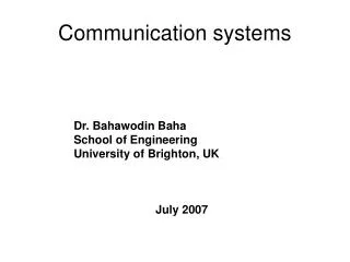
Performance of V-BLAST BER of zero-forcing, V-BLAST and MLD for a (4,6) system using 4-QAM.