Download
1 / 18
180 likes | 290 Views
Point Location. Reading: Chapter 6 of the Textbook Driving Applications Knowing Where You Are in GIS Related Applications Triangulation using Trapezoidal Maps Polygonization of Implicit Surfaces. Knowing Where You Are.

E N D
Point Location • Reading: Chapter 6 of the Textbook • Driving Applications • Knowing Where You Are in GIS • Related Applications • Triangulation using Trapezoidal Maps • Polygonization of Implicit Surfaces M. C. Lin
Knowing Where You Are • Given a map and a query point q specified by its coordinates, find the region of the map containing q. • A map can be treated as a subdivision of the plane into regions, or planar subdivision. • A map can be stored electronically for query preprocessing to answer point location query fast and display the map interactively. M. C. Lin
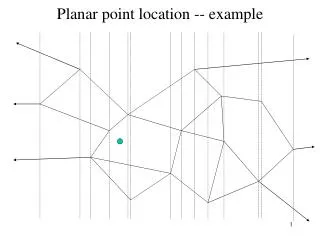
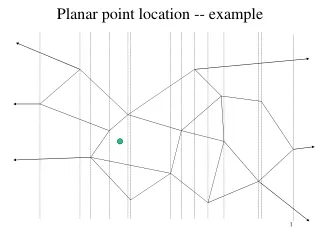
Planar Point Location • Let S be a planar subdivision with n edges. The planar point location problem is to store S in such a way that we can answer: given a query point q, report the face f of S that contains q. If q lies on an edge or a vertex, report so. Partition the plane into vertical slabs. Store the x-coordinates of the vertices in the sorted order in an array. This makes it possible to determine in O(log n) time the slab contains a query point q. M. C. Lin
A Possible Solution • Do a binary search with the x-coordinate of q in the array storing x-coordinates of the subdivision. • Do a binary search within that slab. Given a segment s and the query point q, determine whether q lies above, below or on s. • Query time is good: O(log n). But the storage requirement is high: O(n2)!!! We need a better solution: trapezoidal maps! M. C. Lin
Trapezoidal Maps • We have a set S of n non-crossing line segments, enclosed in a bounding box R, and with no two distinct end points lie on a common vertical line. We call such a set a set of line segments in general position. • The trapezoidal map T(S) of S -- also known as the vertical decomposition or trapezoidal decomposition of S -- is obtained by drawing two vertical extensions from every endpoint p of a segment in S, one going upwards and one going downwards. The extensions stop when they meet another segment of S or the boundary of R. • A face in T(S) is bounded by some edges of T(S) . Some of these edges or sides of a face may be adjacent & collinear. M. C. Lin
Left/Right Edge of Trapezoid • It degenerates to a point, which is the common left/right endpoint of top( ) and bottom(). • It is the lower vertical extension of the left/right endpoint of top( ) that abuts on bottom(). • It is the upper vertical extension of the left/right endpoint of bottom() that abuts on top( ). • It consists of the upper and lower extension of the right endpoint p of a third segment s. These extension abuts on top( ) & bottom() resp. • It’s left/right edge of R. M. C. Lin
Properties of Trapezoidal Maps • The trapezoidal map T(S) of aset S of n line segments in general positions contains at most 6n+4 vertices, at most 3n+1 trapezoids. • The general position assumption is used to established the complexity bounds, but doesn’t affect the algorithm, as will be shown later. • A trapezoid ofT(S) is uniquely defined by its top(), bottom(), leftp() and rightp(); together they store the records of the line segments & endpoints. This structure uses the adjacency of trapezoids to link the subdivision as a whole. M. C. Lin
Trapezoidal Map for Point Location • Use randomized incremental algorithm to construct the trapezoidal map T(S) & point location data structure D. T(S) and D are inter-linked through pointers. • The search structure D is a directed acyclic graph with a single root and exactly one leaf for every trapezoid of T(S). There are 2 types of inner nodes (of out-degree 2): x-nodes, labeled with an endpoint of some segment in S, and y-nodes, labeled with a segment itself. • A query with q starts at the root and proceeds along a directed path to a leaf. At an x-node, the test is “Does q lie to the left or right of the vertical line through endpoint stored at this node?” At a y-node, the test is “Does q lie above or below the segment s stored here?” M. C. Lin
Randomized Incremental Algorithm • Construction of the search structure is incremental: it adds one segment at a time. After each addition, it updates D and T(S). • The order in which the segments are added affects the construction of search structure D. Some results in a good structure and good query time, while others will be bad. But, we are interested in the algorithm that gives us good expected performance, not the best worst-case performance. M. C. Lin
TrapezoidalMap(S) Input: A set S of n non-crossing line segments Output: The trapezoidal map T(S) and a search data structureD for T(S) in a bounding box. 1. Determine a bounding box R that contains all segments of S, and initialize trapezoidal map structure T & search structure D for it 2. Compute a random permutation s1, s2,…, sn of the elements of S. 3. for i 1 to n 4. do Find set 0, 1,…, kof trapezoids in T properly intersected by si 5. Remove 0, 1,…, kfrom T and replace them by new trapezoids that appear because of the insertion of si 6. Remove the leaves of 0, 1,…, kfrom D, and create leaves for the new trapezoids. Link the new leaves to the existing inner nodes by adding some new inner nodes, as explained next. M. C. Lin
FollowSegment(T, si) Input: A trapezoidal map T and a new segment si Output: The sequence 0, 1,…, kof trapezoids intersected by si 1. Let p and q be the left and right endpoint of si 2. Search with p in the search structure to find 0 3. j 0 4. while q lies to the right of rightp(i ) 5. do if rightp(i ) lies above si 6. then Let j+1 be the lower right neighbor of j 7. else Let j+1 be the upper right neighbor of j 8. j j + 1 9. return0, 1,…, j M. C. Lin
Algorithm Analysis • The expected running time is the average running time taken over all n! permutations. The expected size of D is the average sizes of all these resulting search structures. The expected query time for q is the average query time for point q over all runs. • Algorithm TrapezoidalMap computes the trapezoidal map T(S) of a set S of n line segments in general position and a search structure D for T(S) in O(n log n) expected time. The expected size of the search structure D is O(n) and for any query point q the expected query time is O(log n). M. C. Lin
Average Query Time Analysis • The query time for q is linear in the length of the path in D that is traversed when querying with q. It is increased by at most 3 in every iteration based on case analysis. So, 3n is the best possible worst-case bound over all possible insertion order for S. But, we’re interested in average query time w.r.t. all n! possible insertion orders. • Let Xi , for 1 i n, for denote the number of nodes on the path created in i’th iteration. We can express the expected path length as: E[1 i n Xi] = 1 i n E[Xi] M. C. Lin
Average Query Time Analysis Xi 3 E[Xi] 0*(1-Pi ) + 3*Pi E[Xi] 3Pi • q(Si ) disappears if and only if one ofthe top(q(Si )), bottom(q(Si )), leftp(q(Si ) or rightp(q(Si )) disappears with the removal of si. The probability of each event is 1/i. So, Pi = Pr[q(Si )q(Si-1 )] = Pr[q(Si ) T(Si-1 )] 4/i E[1 i n Xi] 1 i n 3Pi 1 i n 12/i = 121 i n 1/i = 12Hn Hn = 1/1 + 1/2 + 1/3 + … + 1/n ln n < Hn < (ln n + 1) Therefore, the query time takes O(log n) M. C. Lin
Expected Size of the Structure • To bound the size, it suffices to bound the number of nodes in D. The leaves in D are in one-to-one correspondence with the trapezoids in T(S), of which there are O(n). Let kibe no. of new trapezoids created in iteration i, due to insertion of segment si: O(n) + E1 i n(number of inner nodes created in iteration i) O(n) + E[1 i n (ki - 1)] = O(n) + 1 i n E[ki] sSi T(Si) (,s) 4 |T(Si )| = O(i) E[ki] = (1/i) sSi T(Si) (,s) O(i)/i = O(1) Thus, the size of the structure is bounded by O(n). M. C. Lin
Expected Construction Time • The time to insert segment siis O(ki) plus the time needed to locate the left endpoint of siin T(Si-1). Use the earlier bound on ki, we get the expected running time for the construction: O(1) + 1 i n { O(log i) + O(E[ki]) } = O(n log n) M. C. Lin
Naïve Assumptions • General position statement assumes no two distinct points have the same x-coordinate. • Assume that a query point never lies on the vertical line of an x-node on its search path, nor on the segment of a y-node. M. C. Lin
Dealing with Degeneracies • Use symbolic perturbation. In effects, use an affine mapping called “shear transform” along the x-axis. • The algorithm does not compute any geometric objects; it never actually computes coordinates of the endpoints. All it does is to apply 2 elementary operations to the input points: • Take 2 distinct points p & q and decides whether q lies to the left, right or on the vertical line through p. • Take 1 of the input segments, specified by p1 & p2, and tests whether a third point q lies above, below, or on this segment. It is only applied when a vertical line through q intersects with this segment. M. C. Lin