Download
1 / 58
580 likes | 715 Views
COSC 3101A - Design and Analysis of Algorithms 9. Knapsack Problem Huffman Codes Introduction to Graphs. Many of these slides are taken from Monica Nicolescu, Univ. of Nevada, Reno, monica@cs.unr.edu. The Knapsack Problem. The 0-1 knapsack problem

E N D
COSC 3101A - Design and Analysis of Algorithms9 Knapsack Problem Huffman Codes Introduction to Graphs Many of these slides are taken from Monica Nicolescu, Univ. of Nevada, Reno, monica@cs.unr.edu
The Knapsack Problem • The 0-1 knapsack problem • A thief rubbing a store finds n items: the i-th item is worth vi dollars and weights wi pounds (vi, wi integers) • The thief can only carry W pounds in his knapsack • Items must be taken entirely or left behind • Which items should the thief take to maximize the value of his load? • The fractional knapsack problem • Similar to above • The thief can take fractions of items COSC3101A
Fractional Knapsack Problem • Knapsack capacity: W • There are n items: the i-th item has value vi and weight wi • Goal: • find xi such that for all 0 xi 1, i = 1, 2, .., n wixi W and xivi is maximum COSC3101A
Fractional Knapsack Problem • Greedy strategy 1: • Pick the item with the maximum value • E.g.: • W = 1 • w1 = 100, v1 = 2 • w2 = 1, v2 = 1 • Taking from the item with the maximum value: Total value taken = v1/w1 = 2/100 • Smaller than what the thief can take if choosing the other item Total value (choose item 2) = v2/w2 = 1 COSC3101A
Fractional Knapsack Problem Greedy strategy 2: • Pick the item with the maximum value per pound vi/wi • If the supply of that element is exhausted and the thief can carry more: take as much as possible from the item with the next greatest value per pound • It is good to order items based on their value per pound COSC3101A
Fractional Knapsack Problem Alg.:Fractional-Knapsack (W, v[n], w[n]) • While w > 0 and as long as there are items remaining • pick item with maximum vi/wi • xi min (1, w/wi) • remove item i from list • w w – xiwi • w – the amount of space remaining in the knapsack (w = W) • Running time: (n) if items already ordered; else (nlgn) COSC3101A
Fractional Knapsack - Example • E.g.: 20 --- 30 50 50 $80 + Item 3 30 20 Item 2 $100 + 20 Item 1 10 10 $60 $60 $100 $120 $240 $6/pound $5/pound $4/pound COSC3101A
Greedy Choice Items: 1 2 3 … j … n Optimal solution: x1 x2 x3 xj xn Greedy solution: x1’ x2’ x3’ xj’ xn’ • We know that: x1’ x1 • greedy choice takes as much as possible from item 1 • Modify the optimal solution to take x1’ of item 1 • We have to decrease the quantity taken from some item j: the new xjis decreased by: (x1’ - x1) w1/wj • Increase in profit: • Decrease in profit: True, since x1 had the best value/pound ratio COSC3101A
Optimal Substructure • Consider the most valuable load that weights at most W pounds • If we remove a weight w of item j from the optimal load • The remaining load must bethe most valuable load weighing at most W – wthat can be taken from the remaining n – 1 items plus wj – w pounds of item j COSC3101A
The 0-1 Knapsack Problem • Thief has a knapsack of capacity W • There are n items: for i-th item value vi and weight wi • Goal: • find xi such that for all xi = {0, 1}, i = 1, 2, .., n wixi W and xivi is maximum COSC3101A
The 0-1 Knapsack Problem • Thief has a knapsack of capacity W • There are n items: for i-th item value vi and weight wi • Goal: • find xi such that for all xi = {0, 1}, i = 1, 2, .., n wixi W and xivi is maximum COSC3101A
50 30 $120 + 20 $100 $220 0-1 Knapsack - Greedy Strategy • E.g.: 50 50 Item 3 30 20 Item 2 $100 + 20 Item 1 10 10 $60 $60 $100 $120 $160 $6/pound $5/pound $4/pound • None of the solutions involving the greedy choice (item 1) leads to an optimal solution • The greedy choice property does not hold COSC3101A
0-1 Knapsack - Dynamic Programming • P(i, w) – the maximum profit that can be obtained from items 1 to i, if the knapsack has size w • Case 1: thief takes item i P(i, w) = • Case 2: thief does not take item i P(i, w) = vi + P(i - 1, w-wi) P(i - 1, w) COSC3101A
first second 0-1 Knapsack - Dynamic Programming P(i, w) = max {vi + P(i - 1, w-wi), P(i - 1, w) } Item i was taken Item i was not taken W w - wi 0: 1 w 0 i-1 i n COSC3101A
P(1, 1) = P(0, 1) = 0 0 P(1, 2) = max{12+0, 0} = 12 P(1, 3) = max{12+0, 0} = 12 P(1, 4) = max{12+0, 0} = 12 max{12+0, 0} = 12 P(1, 5) = P(2, 1)= max{10+0, 0} = 10 P(3, 1)= P(2,1) = 10 P(4, 1)= P(3,1) = 10 P(2, 2)= P(3, 2)= P(2,2) = 12 max{10+0, 12} = 12 P(4, 2)= max{15+0, 12} = 15 P(4, 3)= max{15+10, 22}=25 P(2, 3)= max{10+12, 12} = 22 P(3, 3)= max{20+0, 22}=22 P(2, 4)= max{10+12, 12} = 22 P(3, 4)= max{20+10,22}=30 P(4, 4)= max{15+12, 30}=30 max{20+12,22}=32 P(4, 5)= max{15+22, 32}=37 P(2, 5)= max{10+12, 12} = 22 P(4, 5)= Example: W = 5 P(i, w) = max {vi + P(i - 1, w-wi), P(i - 1, w) } 0 1 2 3 4 5 0 12 12 12 12 1 10 12 22 22 22 2 10 12 22 30 32 3 10 15 25 30 37 4 COSC3101A
Item 4 • Item 2 • Item 1 Reconstructing the Optimal Solution 0 1 2 3 4 5 0 12 12 0 12 12 1 10 12 22 22 22 2 10 12 22 30 32 3 10 15 25 30 37 4 • Start at P(n, W) • When you go left-up item i has been taken • When you go straight up item i has not been taken COSC3101A
Optimal Substructure • Consider the most valuable load that weights at most W pounds • If we remove item j from this load • The remaining load must be the most valuable load weighing at most W – wjthat can be taken from the remaining n – 1 items COSC3101A
Overlapping Subproblems P(i, w) = max {vi + P(i - 1, w-wi), P(i - 1, w) } w W 0: 1 0 i-1 i n E.g.: all the subproblems shown in grey may depend on P(i-1, w) COSC3101A
Huffman Codes • Widely used technique for data compression • Assume the data to be a sequence of characters • Looking for an effective way of storing the data COSC3101A
Huffman Codes • Idea: • Use the frequencies of occurrence of characters to build a optimal way of representing each character • Binary character code • Uniquely represents a character by a binary string COSC3101A
Fixed-Length Codes E.g.: Data file containing 100,000 characters • 3 bits needed • a = 000, b = 001, c = 010, d = 011, e = 100, f = 101 • Requires: 100,000 3 = 300,000 bits COSC3101A
Variable-Length Codes E.g.: Data file containing 100,000 characters • Assign short codewords to frequent characters and long codewords to infrequent characters • a = 0, b = 101, c = 100, d = 111, e = 1101, f = 1100 • (45 1 + 13 3 + 12 3 + 16 3 + 9 4 + 5 4) 1,000 = 224,000 bits COSC3101A
Prefix Codes • Prefix codes: • Codes for which no codeword is also a prefix of some other codeword • Better name would be “prefix-free codes” • We can achieve optimal data compression using prefix codes • We will restrict our attention to prefix codes COSC3101A
Encoding with Binary Character Codes • Encoding • Concatenate the codewords representing each character in the file • E.g.: • a = 0, b = 101, c = 100, d = 111, e = 1101, f = 1100 • abc = 0 101 100 = 0101100 COSC3101A
Decoding with Binary Character Codes • Prefix codes simplify decoding • No codeword is a prefix of another the codeword that begins an encoded file is unambiguous • Approach • Identify the initial codeword • Translate it back to the original character • Repeat the process on the remainder of the file • E.g.: • a = 0, b = 101, c = 100, d = 111, e = 1101, f = 1100 • 001011101 = 0 =aabe 0 101 1101 COSC3101A
100 100 0 1 0 1 55 86 14 a: 45 0 1 1 0 0 30 25 58 28 14 0 1 1 0 0 1 0 1 0 1 14 c: 12 b: 13 d: 16 a: 45 b: 13 c: 12 d: 16 e: 9 f: 5 0 1 f: 5 e: 9 Prefix Code Representation • Binary tree whose leaves are the given characters • Binary codeword • the path from the root to the character, where 0 means “go to the left child” and 1 means “go to the right child” • Length of the codeword • Length of the path from root to the character leaf (depth of node) COSC3101A
Optimal Codes • An optimal code is always represented by a full binary tree • Every non-leaf has two children • Fixed-length code is not optimal, variable-length is • How many bits are required to encode a file? • Let C be the alphabet of characters • Let f(c) be the frequency of character c • Let dT(c) be the depth of c’s leaf in the tree T corresponding to a prefix code the cost of tree T COSC3101A
f: 5 e: 9 c: 12 b: 13 d: 16 a: 45 Constructing a Huffman Code • A greedy algorithm that constructs an optimal prefix code called a Huffman code • Assume that: • C is a set of n characters • Each character has a frequency f(c) • The tree T is built in a bottom up manner • Idea: • Start with a set of |C| leaves • At each step, merge the two least frequent objects: the frequency of the new node = sum of two frequencies • Use a min-priority queue Q, keyed on f to identify the two least frequent objects COSC3101A
14 c: 12 b: 13 d: 16 a: 45 f: 5 e: 9 c: 12 b: 13 d: 16 a: 45 0 1 f: 5 e: 9 30 d: 16 a: 45 a: 45 14 14 14 14 25 25 25 25 0 1 0 1 1 0 0 1 d: 16 f: 5 f: 5 f: 5 f: 5 e: 9 e: 9 e: 9 e: 9 c: 12 c: 12 c: 12 c: 12 b: 13 b: 13 b: 13 b: 13 0 1 100 1 0 55 a: 45 1 0 55 a: 45 0 1 30 30 1 0 1 0 1 1 0 0 d: 16 d: 16 1 0 0 1 Example COSC3101A
O(n) O(nlgn) Building a Huffman Code Alg.: HUFFMAN(C) • n C • Q C • fori 1ton – 1 • do allocate a new node z • left[z] x EXTRACT-MIN(Q) • right[z] y EXTRACT-MIN(Q) • f[z] f[x] + f[y] • INSERT (Q, z) • return EXTRACT-MIN(Q) Running time: O(nlgn) COSC3101A
Greedy Choice Property Lemma:Let C be an alphabet in which each character c C has frequency f[c]. Let x and y be two characters in C having the lowest frequencies. Then, there exists an optimal prefix code for C in which the codewords for x and y have the same length and differ only in the last bit. COSC3101A
Proof of the Greedy Choice • Idea: • Consider a tree T representing an arbitrary optimal prefix code • Modify T to make a tree representing another optimal prefix code in which x and y will appear as sibling leaves of maximum depth • The codes of x and y will have the same length and differ only in the last bit COSC3101A
T’ T’’ a x a b y y a x x b b y Proof of the Greedy Choice (cont.) • a, b – two characters, sibling leaves of maximum depth in T • Assume: f[a] f[b] and f[x] f[y] • f[x] and f[y] are the two lowest leaf frequencies, in order • f[x] f[a] and f[y] f[b] • Exchange the positions of a and x (T’) and of b and y (T’’) T COSC3101A
x a a y y b x a x b y b Proof of the Greedy Choice (cont.) T T’ T’’ B(T) – B(T’) = = f[x]dT(x) + f[a]dT(a) – f[x]dT’(x) – f[a]dT’(a) = f[x]dT(x) + f[a]dT(a) – f[x]dT(a) – f[a]dT (x) = (f[a] - f[x]) (dT(a) - dT(x)) 0 ≥ 0 x is a minimum frequency leaf ≥ 0 a is a leaf of maximum depth COSC3101A
x a a y y b x x a b b y Proof of the Greedy Choice (cont.) B(T) – B(T’) 0 Similarly, exchanging y and b does not increase the cost B(T’) – B(T’’) 0 • B(T’’) B(T) and since T is optimal B(T) B(T’’) • B(T) = B(T’’) T’’ is an optimal tree, in which x and y are sibling leaves of maximum depth T T’ T’’ COSC3101A
Discussion • Greedy choice property: • Building an optimal tree by mergers can begin with the greedy choice: merging the two characters with the lowest frequencies • The cost of each merger is the sum of frequencies of the two items being merged • Of all possible mergers, HUFFMAN chooses the one that incurs the least cost COSC3101A
Graphs • Applications that involve not only a set of items, but also the connections between them • Maps • Hypertexts • Circuits • Schedules • Transactions • Matching • Computer Networks COSC3101A
2 2 1 1 2 1 3 4 3 4 3 4 Graphs - Background Graphs = a set of nodes (vertices) with edges (links) between them. Notations: • G = (V, E) - graph • V = set of vertices V = n • E = set of edges E = m Directed graph Undirected graph Acyclic graph COSC3101A
2 1 3 4 2 1 2 1 9 4 8 6 3 3 4 7 4 Other Types of Graphs • A graph is connected if there is a path between every two vertices • A bipartite graph is an undirected graph G = (V, E) in which V = V1 + V2 and there are edges only between vertices in V1 and V2 Connected Not connected COSC3101A
2 1 3 5 4 Graph Representation • Adjacency list representation of G = (V, E) • An array of V lists, one for each vertex in V • Each list Adj[u] contains all the vertices v such that there is an edge between u and v • Adj[u] contains the vertices adjacent to u (in arbitrary order) • Can be used for both directed and undirected graphs 1 2 3 4 5 Undirected graph COSC3101A
2 1 2 1 3 5 4 3 4 Properties of Adjacency-List Representation • Sum of the lengths of all the adjacency lists • Directed graph: • Edge (u, v) appears only once in u’s list • Undirected graph: • u and v appear in each other’s adjacency lists: edge (u, v) appears twice Directed graph E 2 E Undirected graph COSC3101A
2 1 2 1 3 5 4 3 4 Properties of Adjacency-List Representation • Memory required • (V + E) • Preferred when • the graph is sparse: E << V 2 • Disadvantage • no quick way to determine whether there is an edge between node u and v • Time to list all vertices adjacent to u: • (degree(u)) • Time to determine if (u, v) E: • O(degree(u)) Undirected graph Directed graph COSC3101A
0 1 0 1 0 0 1 1 1 1 2 1 0 1 0 1 0 3 1 0 1 0 1 5 4 1 1 0 0 1 Graph Representation • Adjacency matrix representation of G = (V, E) • Assume vertices are numbered 1, 2, … V • The representation consists of a matrix A V x V : • aij = 1 if (i, j) E 0 otherwise 1 2 3 4 5 Matrix A is symmetric: aij = aji A = AT 1 2 3 4 Undirected graph 5 COSC3101A
Properties of Adjacency Matrix Representation • Memory required • (V2), independent on the number of edges in G • Preferred when • The graph is dense E is close to V 2 • We need to quickly determine if there is an edge between two vertices • Time to list all vertices adjacent to u: • (V) • Time to determine if (u, v) E: • (1) COSC3101A
Weighted Graphs • Weighted graphs = graphs for which each edge has an associated weight w(u, v) w:E R, weight function • Storing the weights of a graph • Adjacency list: • Store w(u,v) along with vertex v in u’s adjacency list • Adjacency matrix: • Store w(u, v) at location (u, v) in the matrix COSC3101A
Searching in a Graph • Graph searching = systematically follow the edges of the graph so as to visit the vertices of the graph • Two basic graph searching algorithms: • Breadth-first search • Depth-first search • The difference between them is in the order in which they explore the unvisited edges of the graph • Graph algorithms are typically elaborations of the basic graph-searching algorithms COSC3101A
Breadth-First Search (BFS) • Input: • A graph G = (V, E) (directed or undirected) • A source vertex s V • Goal: • Explore the edges of G to “discover” every vertex reachable from s, taking the ones closest to s first • Output: • d[v] = distance (smallest # of edges) from s to v, for all v V • A “breadth-first tree” rooted at s that contains all reachable vertices COSC3101A
2 1 3 5 4 11 7 6 9 12 7 Breadth-First Search (cont.) • Discover vertices in increasing order of distance from the source s – search in breadth not depth • Find all vertices at 1 edge from s, then all vertices at 2 edges from s, and so on COSC3101A
2 2 2 1 1 1 3 3 3 5 5 5 4 4 4 Breadth-First Search (cont.) • Keeping track of progress: • Color each vertex in either white, gray or black • Initially, all vertices are white • When being discovered a vertex becomes gray • After discovering all its adjacent vertices the node becomes black • Use FIFO queue Q to maintain the set of gray vertices source COSC3101A
2 1 3 5 4 Breadth-First Tree • BFS constructs a breadth-first tree • Initially contains the root (source vertex s) • When vertex v is discovered while scanning the adjacency list of a vertex u vertex v and edge (u, v) are added to the tree • u is the predecessor (parent) of v in the breadth-first tree • A vertex is discovered only once it has at most one parent source COSC3101A