Download
1 / 19
190 likes | 350 Views
Hyperspectral Infrared Water Vapor Radiance Assimilation. James Jung Contributions From: Paul Van Delst, Fanglin Yang, Chris Barnet, John Le Marshall, Lars Peter Riishojgaard and many others. Water Vapor Radiance Assimilation. Problems Innovations do not have a normal distribution

E N D
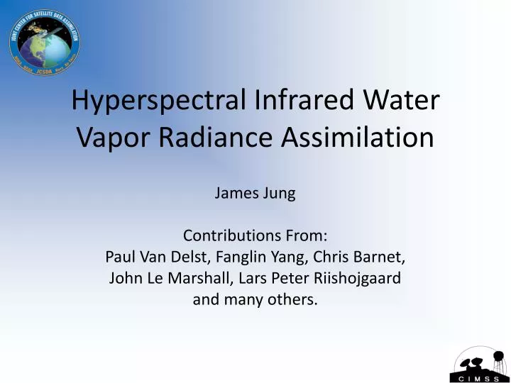
Hyperspectral Infrared Water Vapor Radiance Assimilation James Jung Contributions From: Paul Van Delst, Fanglin Yang, Chris Barnet, John Le Marshall, Lars Peter Riishojgaard and many others.
Water Vapor Radiance Assimilation • Problems • Innovations do not have a normal distribution • Use q, log(q) or pseudo RH • All have +/- • Multivariate problem • T and q are both unknown • Non-linearity • Symptoms • Increased penalty • Decreased convergence • Unstable moisture field • Supersaturation • Negative moisture • Precipitation spin down
GSI Software Modifications • Q < 1.0e-7, reset to 1.0e-7 before each outer loop and analysis output • Minimal impact • Q > = 1.0e-7 for CRTM vice 1.0e-6 • Minimal impact • Supersaturation is reset to saturation during initial read (to properly compute heights), before each outer loop, and analysis output. • Substantial impact • ** REVIEW RH BACKGROUND ERROR ** • Adjust factqmax and factqmin to slow production of negative and supersaturated Q. • Adjust conventional observation errors
GSI Software Modifications Factqmax and factqmin are inflation terms which add to the cost function when negative water vapor or supersaturation occur in the inner loops. • Stratospheric components of the AIRS and IASI water vapor jacobians may need to be adjusted based on model top and vertical resolution. • Weak water vapor lines in surface and CO2 channels. • Near absorption lines in water vapor region. • Needs to be tuned for each model • Model generated supersaturation • Background Error and factqmax/factqmin will degrade convergence. • Will need to re-compute bias corrections for any water vapor radiances being used.
Water Vapor Radiances • Use the gross error check to limit the response for all water vapor channels. • Adjusted gross error check 4.5 -> 0.9 [K] (AIRS and IASI) • Adjusted gross error check 4.5 -> 1.5 [K] (HIRS and GOES) • Adjusted gross error check 6.0 -> 3.0 [K] (MW sensors) • Assumes clear sky conditions. • Adjusted assimilation weights closer to the noise equivalent delta temperature (nedt). • 233 total, 68 water vapor IASI channels • 53 tropospheric (off-line) • 31 stratospheric (on-line) • 121 total, 38 water vapor AIRS channels • 29 tropospheric (off-line) • 9 stratospheric (on-line) • All HIRS, GOES, AMSU-B and MHS water vapor channels are used.
Effects • Less observations per channel used wrt using the original gross error check. • ~70% reduction initially • ~20% reduction in final analysis • Most observations pass QC on second outer loop • Better temperature profile (?) • Water vapor channels now have similar characteristics to temperature channels • Convergence improved • Penalty improved • Smaller initial changes to the moisture field, greater changes over time • Each assimilation cycle changes are about an order of magnitude less than the model values • Most changes occurring in the mid- and upper Troposphere
Vertical RMS fit to Raobs Solid Lines = control Dashed Lines = experiment Red = Background Black = Analysis
Consistent improvements with respect to rawinsaondes are realized in all four seasons Solid Lines = control Dashed Lines = experiment Red = Background Black = Analysis
500 hPa Time series of RMS fit to RAOBS control experiment Improvements in the analysis and 6 hour forecast
Analysis Differences of Relative Humidity at selected levels Experiment Red < Green > 1 Mar – 31 May 2010
Analysis Differences of Precipitable Water 1 Mar – 31 May 2010 1 Jun – 31 Aug 2010 1 Sep – 30 Nov 2010 1 Dec 2010 – 28 Feb 2011
6 hour accumulated precipitation differences for each season 1 Mar – 31 May 2010 1 Jun – 31 Aug 2010 1 Sep – 30 Nov 2010 1 Dec 2010 – 28 Feb 2011
Summary • Water vapor statistics show • Improvements with respect to rawinsondes are noted in the analysis and 6 hour forecast. • Upper troposphere is dryer. • Tropics have marginally higher PW • Polar regions are generally dryer. • Rainfall differences are noted up to 12 hours in all four seasons • Other seasons statistics are similar • Non water vapor statistics are mostly neutral (not shown) • Anomaly correlations. • Wind, temperature, etc. fits to observations.
Stratosphere Water Vapor Assimilation Overview • Using infrared radiances to “estimate” stratospheric moisture. • These are moisture ESTIMATES • Observations are not available • Derived from jacobian tails • Uses a nudging approach • 3 Sources of information • IASI (dominant) • AIRS • GPS-RO
Vertical Distribution of Water Vapor Standard longitudinal average (not ln(q)) Single assimilation cycle .
Horizontal Distribution of Water Vapor Colors are x10-6 [Kg/Kg]
Analysis and forecast stratosphere temperature fits to rawinsondes for March-April-May 2010 Control Experiment
Stratosphere Forecast Temperature drift comparison (Forecast – Analysis) at 20 and 30 hPa experiment experiment control control March-April-May 2010
Summary • Using hyperspectral IR radiances, it is possible to generate reasonable estimates of specific humidity in the stratosphere. • Qualitative stratospheric water vapor analysis with other sensors show: • Equal to slightly wetter with respect to HALOE. • Dryer with respect to SAGE II, Aura MLS, and MIPAS. • Stratosphere water vapor assimilation requires a long spinup time • 2+ months after being initialized to > 3.0e-6 [Kg/Kg] • Rawinsonde comparisons suggest: • A slightly cooler stratospheric temperature (cold bias). • A reduced stratospheric temperature drift with time. • Stratospheric temperature comparisons with its own analysis are improved through 48 hours.