Download
1 / 39
410 likes | 911 Views
Introduction to Management Science 8th Edition by Bernard W. Taylor III. Chapter 7 Linear Programming: Computer Solution and Sensitivity Analysis. Chapter Topics. Computer Solution Microsoft Excel’s “Solver” module QM for Excel QM for Windows Sensitivity Analysis Done “by hand”

E N D
Introduction to Management Science 8th Edition by Bernard W. Taylor III Chapter 7 Linear Programming: Computer Solution and Sensitivity Analysis Chapter 7 - Linear Programming: Computer Solution and Sensitivity Analysis
Chapter Topics • Computer Solution • Microsoft Excel’s “Solver” module • QM for Excel • QM for Windows • Sensitivity Analysis • Done “by hand” • Using Microsoft Excel’s “Solver” module • QM for Excel • QM for Windows Chapter 7 - Linear Programming: Computer Solution and Sensitivity Analysis
Computer Solution • Early linear programming used lengthy manual mathematical solution procedure called the Simplex Method (See CD-ROM Module A). • Steps of the Simplex Method have been programmed in software packages designed for linear programming problems. • Many such packages available currently. • Used extensively in business and government. • Text focuses on Excel Spreadsheets and QM for Windows. Chapter 7 - Linear Programming: Computer Solution and Sensitivity Analysis
Beaver Creek Pottery Example Excel Spreadsheet – Data Screen (1 of 5) Exhibit 7.1 Chapter 7 - Linear Programming: Computer Solution and Sensitivity Analysis
Click on “Options” and then on “Assume Linear Models” ! Beaver Creek Pottery Example “Solver” Parameter Screen(2 of 5) Exhibit 7.2 Chapter 7 - Linear Programming: Computer Solution and Sensitivity Analysis
Beaver Creek Pottery Example Adding Model Constraints (3 of 5) Exhibit 7.3 Chapter 7 - Linear Programming: Computer Solution and Sensitivity Analysis
Running “Solver” will iterativelyvary B10 and B11 to reduce theslack in G10 & G11. Beaver Creek Pottery Example Solution Screen (4 of 5) Exhibit 7.4 Chapter 7 - Linear Programming: Computer Solution and Sensitivity Analysis
Beaver Creek Pottery Example Answer Report (5 of 5) This report is generated only when one clicks on “Options” and then on “assume Linear Models” when setting up the “Solver” calculation ! Exhibit 7.5 Chapter 7 - Linear Programming: Computer Solution and Sensitivity Analysis
Linear Programming Problem Standard Form • Standard form requires all variables in the constraint equations to appear on the left of the inequality (or equality) and all numeric values to be on the right-hand side. • Examples: • x3 x1 + x2 must be converted to x3 - x1 - x2 0 • x1/(x2 + x3) 2 becomes x1 2 (x2 + x3)and then x1 - 2x2 - 2x3 0 Chapter 7 - Linear Programming: Computer Solution and Sensitivity Analysis
Beaver Creek Pottery Example QM for Windows – Data Screen(1 of 3) Exhibit 7.6 Chapter 7 - Linear Programming: Computer Solution and Sensitivity Analysis
Beaver Creek Pottery Example Model Solution Screen(2 of 3) Exhibit 7.7 Chapter 7 - Linear Programming: Computer Solution and Sensitivity Analysis
Beaver Creek Pottery Example Graphical Solution Screen(3 of 3) Exhibit 7.8 Chapter 7 - Linear Programming: Computer Solution and Sensitivity Analysis
Beaver Creek Pottery Example Sensitivity Analysis(1 of 4) • Sensitivity analysis determines the effect on optimal solutions of changes in parameter values of the objective function and constraint equations. • Changes may be reactions to anticipated uncertainties in the parameters or to new or changed information concerning the model. Chapter 7 - Linear Programming: Computer Solution and Sensitivity Analysis
Beaver Creek Pottery Example Sensitivity Analysis(2 of 4) Maximize Z = $40x1 + $50x2 subject to: 1x1 + 2x2 40 4x1 + 3x2 120 x1, x2 0 Figure 7.1 Optimal Solution Point Chapter 7 - Linear Programming: Computer Solution and Sensitivity Analysis
Changed from $40 Old optimal solution Beaver Creek Pottery Example Change x1 Objective Function Coefficient (3 of 4) Maximize Z = $100x1 + $50x2 subject to: 1x1 + 2x2 40 4x1 + 3x2 120 x1, x2 0 New optimal solution Figure 7.2 Changing the x1 Objective Function Coefficient Chapter 7 - Linear Programming: Computer Solution and Sensitivity Analysis
Changed from $50 Beaver Creek Pottery Example Change x2 Objective Function Coefficient (4 of 4) Old optimal solution Maximize Z = $40x1 + $100x2 subject to: 1x1 + 2x2 40 4x1 + 3x2 120 x1, x2 0 Figure 7.3 Changing the x2 Objective Function Coefficient Chapter 7 - Linear Programming: Computer Solution and Sensitivity Analysis
Objective Function Coefficient Sensitivity Range (1 of 3) • The sensitivity range for an objective function coefficient is the range of values over which the current optimal solution point will remain optimal. • The sensitivity range for the xi coefficient, i.e., of ci, the coefficient of xi in the objective function, Z: Z = c1 x1 + c2 x2 + c3 x3 + …The sensitivity range is the interval within which a single coefficient, one at a time, can be varied without changing the optimal value of the objective function. (Although there do appear multiple alternate optimal values.) Chapter 7 - Linear Programming: Computer Solution and Sensitivity Analysis
– 66.67/50 = – 4/3 – 25/50 = – 1/2 Objective Function Coefficient Sensitivity Range for c1 and c2 (2 of 3) objective function Z = $40x1 + $50x2 sensitivity range for: x1: 25 c1 66.67 x2: 30 c2 80 Slope = – c1/c2 Figure 7.4 Determining the Sensitivity Range for c1 Chapter 7 - Linear Programming: Computer Solution and Sensitivity Analysis
Objective Function Coefficient Fertilizer Cost Minimization Example (3 of 3) Minimize Z = $6x1 + $3x2 subject to: 2x1 + 4x2 16 4x1 + 3x2 24 x1, x2 0 sensitivity ranges: 4 c1 0 c2 4.5 Figure 7.5 Fertilizer Cost Minimization Example Chapter 7 - Linear Programming: Computer Solution and Sensitivity Analysis
Objective Function Coefficient Ranges Excel “Solver” Results Screen (1 of 3) Exhibit 7.9 Chapter 7 - Linear Programming: Computer Solution and Sensitivity Analysis
Objective Function Coefficient Ranges Beaver Creek Example Sensitivity Report (2 of 3) This report is generated only when one clicks on “Options” and then on “assume Linear Models” when setting up the “Solver” calculation ! Exhibit 7.10 Chapter 7 - Linear Programming: Computer Solution and Sensitivity Analysis
Objective Function Coefficient Ranges QM for Windows Sensitivity Range Screen (3 of 3) Exhibit 7.11 Chapter 7 - Linear Programming: Computer Solution and Sensitivity Analysis
Changes in Constraint Quantity Values Sensitivity Range (1 of 4) • The sensitivity range for a right-hand-side value is the range of values over which the quantity values can change without changing the solution variable mix, including slack variables. Chapter 7 - Linear Programming: Computer Solution and Sensitivity Analysis
Consider the Labor Constraintchanging from q1=40 to q1=60 Changes in Constraint Quantity Values Increasing the Labor Constraint (2 of 4) Maximize Z = $40x1 + $50x2 subject to: 1x1 + 2x2 40 4x1 + 3x2 120 x1, x2 0 Figure 7.6 Increasing the Labor Constraint Quantity Chapter 7 - Linear Programming: Computer Solution and Sensitivity Analysis
Changes in Constraint Quantity Values Sensitivity Range for Labor Constraint (3 of 4) Sensitivity range for: 30 q1 80 hr The “maximal” and the “minimal”values of the Labor ConstraintQuantity: Figure 7.7 Determining the Sensitivity Range for Labor Quantity Chapter 7 - Linear Programming: Computer Solution and Sensitivity Analysis
Changes in Constraint Quantity Values Sensitivity Range for Clay Constraint (4 of 4) Sensitivity range for: 60 q2 160 lb The amount of change in Zfor a unit change in a constraintquantity is that quantity’s dual(shadow) price. Figure 7.8 Determining the Sensitivity Range for Clay Quantity Chapter 7 - Linear Programming: Computer Solution and Sensitivity Analysis
Constraint Quantity Value Ranges by Computer Excel Sensitivity Range for Constraints (1 of 2) Exhibit 7.12 Chapter 7 - Linear Programming: Computer Solution and Sensitivity Analysis
Constraint Quantity Value Ranges by Computer QM for Windows Sensitivity Range (2 of 2) Exhibit 7.13 Chapter 7 - Linear Programming: Computer Solution and Sensitivity Analysis
Other Forms of Sensitivity Analysis Topics (1 of 4) • Changing individual constraint parameters • One at a time! • Adding new constraints • …or modifying the existing ones by changing the relatione.g., by changing ‘≤’ into ‘=’ to enforce saturation (no slack) • Adding new variables • Makes the problem more complicated, but also more versatile Chapter 7 - Linear Programming: Computer Solution and Sensitivity Analysis
Figure 7.9 Changing the x1 Coefficient in the Labor Constraint Other Forms of Sensitivity Analysis Changing a Constraint Parameter (2 of 4) Maximize Z = $40x1 + $50x2 subject to: 1x1 + 2x2 40 4x1 + 3x2 120 x1, x2 0 Chapter 7 - Linear Programming: Computer Solution and Sensitivity Analysis
Other Forms of Sensitivity Analysis Adding a New Constraint (3 of 4) Adding a new constraint to Beaver Creek Model: 0.20x1+ 0.10x2 5 hours for packaging Original solution: 24 bowls, 8 mugs, $1,360 profit Exhibit 7.13 Chapter 7 - Linear Programming: Computer Solution and Sensitivity Analysis
Other Forms of Sensitivity Analysis Adding a New Variable (4 of 4) Adding a new variable to the Beaver Creek model, x3, a third product, cups Maximize Z = $40x1 + 50x2 + 30x3 subject to: x1 + 2x2 + 1.2x3 40 hr of labor 4x1 + 3x2 + 2x3 120 lb of clay x1, x2, x3 0 Solving model shows that change has no effect on the original solution (i.e., the model is not sensitive to this change). Chapter 7 - Linear Programming: Computer Solution and Sensitivity Analysis
Shadow Prices (Dual Values) • Defined as the marginal value of one additional unit of resource. • Also defined (earlier) as: “the amount of change in the objective function for a unit change in a constraint quantity.” • That is, by allotting one extra unit of a resource/constraint quantity (denoted qi), the objective function changes by the shadow price or that resource. • The sensitivity range for a constraint quantity value is also the range over which the shadow price is valid. Chapter 7 - Linear Programming: Computer Solution and Sensitivity Analysis
Excel Sensitivity Report for Beaver Creek Pottery Shadow Prices Example (1 of 2) Maximize Z = $40x1 + $50x2 subject to: x1 + 2x2 40 hr of labor 4x1 + 3x2 120 lb of clay x1, x2 0 For every additional hour of labor,the profit will increase by $16.Labor can be increased from 40 to40 + 40 = 80, before the solution(x1,x2) changes. Exhibit 7.14 Chapter 7 - Linear Programming: Computer Solution and Sensitivity Analysis
Excel Sensitivity Report for Beaver Creek Pottery Solution Screen (2 of 2) Exhibit 7.15 Chapter 7 - Linear Programming: Computer Solution and Sensitivity Analysis
Example Problem Problem Statement (1 of 3) • Two airplane parts: no.1 and no. 2. • Three manufacturing stages: stamping, drilling, milling. • Decision variables: x1 (number of part no.1 to produce) x2 (number of part no.2 to produce) • Model: Maximize Z = $650x1 + 910x2 subject to: 4x1 + 7.5x2 105 (stamping,hr) 6.2x1 + 4.9x2 90 (drilling, hr) 9.1x1 + 4.1x2 110 (finishing, hr) x1, x2 0 Chapter 7 - Linear Programming: Computer Solution and Sensitivity Analysis
Example Problem Graphical Solution (2 of 3) Maximize Z = $650x1 + $910x2 subject to: 4x1 + 7.5x2 105 6.2x1 + 4.9x2 90 9.1x1 + 4.1x2 110 x1, x2 0 s1 = 0, s2 = 0, s3 = 11.35 hr Coefficient sensitivity:485.33 c1 1,151.43 Quantity sensitivity: 89.10 q1 137.76 Figure 7.10 Graphical Solution Chapter 7 - Linear Programming: Computer Solution and Sensitivity Analysis
Example Problem Excel Solution (3 of 3) Exhibit 7.16 Chapter 7 - Linear Programming: Computer Solution and Sensitivity Analysis
Chapter 7 - Linear Programming: Computer Solution and Sensitivity Analysis