Download
1 / 52
520 likes | 621 Views
This study focuses on proving reachability in linked data structures, offering solutions for partial and total program correctness, memory safety, and data structure invariants while addressing the challenges of complexity in reasoning and undecidability.

E N D
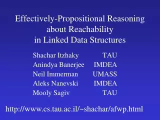
Effectively-Propositional Reasoning about Reachabilityin Linked Data Structures TAU IMDEA UMASS IMDEA TAU Shachar Itzhaky Anindya Banerjee Neil Immerman Aleks Nanevski Mooly Sagiv http://www.cs.tau.ac.il/~shachar/afwp.html
Motivation • Proving presence (absence) of pointer paths between memory allocated objects in a given program • Partial program correctness • Memory safety • Absence of memory leaks • Data structure invariants • Acylicity, Sortedness • Total program correctness • Program equivalence
Program Termination {x <n*> y} n n n n x null y traverse(Node x, Node y) { for (t =x; t != y ; t = t.n) { … } }
Disjoint Parallelism {: null (h<n*> k<n*> )} n n n n n n n h null x k null y • for (x =h; x != null; x = x.n) { • … • } • for (y=k; y != null; y = y.n) { • … • }
Challenges • Complexity of reasoning about reachability assertions • Undecidability of reachability • [Inferring reachability properties from the code] "there is a mismatch between the simple intuitions about the way pointer operations work and the complexity of their axiomatic treatments" O'Hearn, Reynolds, Yang [CSL 2001]
Link list manipulations are simple • Simple to reason about correctness • Small counterexamples • “Simple” invariants • Alternation Free + Reachability “” **
EA(**) formulasBernays-Schönfinkel-Ramsey • t ::= var | constant (Terms) • ap ::= t1 = t2 | r(t1,t2, …, tn) • qf ::= ap | qf1qf2 | qf1 qf2 | qf • ea ::= 1, 2, n: 1, 2, m: qf • Effectively Propositional • Skolimization yields finite models • EQ-satisfiable to a propositional formula • Support from Z3
EA() formulasBernays-Schönfinkel-Ramsey 1, 2, : 1 : r(1, 1) r(1, 2) =sat 1 : r(c1, 1) r(1, c2) =sat(r(c1, c1) r(c1, c2)) (r(c1, c2) r(c2, c2)) =sat (P11 P12) (P12 P22)
Alternation Free Reachability (AFR) • “Extended subset” of EA • Closed under negation • t ::= var | constant (Terms) • ap ::= t1 = t2 | r(t1,t2, …, tn) | t1 <f*> t2 (Reachability via sequences of f’s) (exists k: fk (t1)=t2 ) • qf ::= qf | qf1qf2 | qf1 qf2 | qf • e ::= 1, 2,…, n: qfa: ::= 1, 2,…, m: qf • afR ::= e | a | afR1 afR2 | afR1 afR2
AFR Program Properties n* • Acylicity • , : <n+> <n+> • , : <n*> <n*> = • Acyclic list with a head h • , : h<n*> h<n*> <n*> <n*> = • Sorted segment • ,: <n*> data n* h n* n* n* v u u v
AFR Program Properties f * • Doubly linked lists • , : <f *> <b*> • Disjoint lists with heads h and k • : null (h<n*> k<n*> ) b* h 1 n* k 2
List Reversal (isolatd) {ac [h]:h <n*>} Node reverse(Node h) { Node c = h; Node d = null; while (c != null) { Node t = c.next; c.next = d; d = c; c = t; } return d } h n* d n* n* n null null n n* n* n* <n*> <n*>
Invariant List Reversal (isolatd) {ac [h]:h <n*>} Node reverse(Node h) { Node c = h; Node d = null; while (c != null) { Node t = c.next; c.next = d; d = c; c = t; } return d } d<n*> <n*> <n*> c <n*> (<n*> <n*>) d<n*> I= , : h n* d c n* n* n n null n null n* n* n*
List Reversal (isolated) {ac [h]:h <n*>} Node reverse(Node h) { Node c = h; Node d = null; while {I} (c != null) { Node t = c.next; c.next = d; d = c; c = t; } return d } d<n*> <n*> <n*> c <n*> (<n*> <n*>) d<n*> I= , : {ac[d] , : <n*> <n*>}
List Reversal (isolated) {ac [h]:h <n*>} Node reverse(Node h) { Node c = h; Node d = null; while {I} (c != null) { Node t = c.next; c.next = d; d = c; c = t; } return d } d<n*> <n*> <n*> c <n*> (<n*> <n*>) d<n*> I= , : {ac[d] , : <n*> <n*> :d <n*>}
List Reversal (ownership) {, :h <n*> <n*> h <n*> } Node reverse(Node h) { Node c = h; Node d = null; while {I} (c != null) { Node t = c.next; c.next = d; d = c; c = t; } return d }
List Reversal (ownership) Case 1: h<n*> h<n*> h n* d n* n* n null null n n* n* n* <n*> <n*>
List Reversal (ownership) Case 2: h<n*> h<n*> n*, n* h d n* n null null n n* <n*> <n*>
List Reversal (ownership) Case 3: h<n*> h<n*> h d n* n* n null null n n* n* <n*> false
List Reversal (ownership) Case 4: h<n*> h<n*> h= d n* n null n*, n* n n* null <n*> <n*>h=
List Reversal (ownership) {ac [h] , :h <n*> <n*> h <n*> } Node reverse(Node h) { Node c = h; Node d = null; while (c != null) { Node t = c.next; c.next = d; d = c; c = t; } return d; } h<n*> h<n*> <n*> h<n*> h<n*> <n*> , :<n*> h<n*> h<n*> false h<n*> h<n*> <n*>h=
Why AFR? • Represents the invariants of simple linked list manipulations • Closed under , , , • Finite model property • Decidable for satisfiability/validity • AFR AF • Can be reduced to a propositional formula • SAT solver is complete for verification/falsification
AFR AF • Introduce an auxiliary relation n* • t[ <n*>] =n*(, ) • Completely axiomatize n* by an AF formula linOrd=, : n*(, ) n*(, ) = , , : n*(, ) n*(, ) n*(, ) , , : n*(, ) n*(, ) (n*(, ) n*(, )) • is satisfiable (linOrd t[]) is satisfiable • AF formulas have finite model
Inverting n* n • Every finite model in which n* satisfies the order requirements:linOrd=, : n*(, ) n*(, ) = , , : n*(, ) n*(, ) n*(, ) , , : n*(, ) n*(, ) (n*(, ) n*(, )) • n* uniquely determines n
Inverting n* n n* n* n* u v n* n* n* n* n* y n* n* n* x w n* n* n* <n+> <n*>
Inverting n* n n+ n u v n n+ n+ n+ n+ n n+ y n+ n+ n+ x w n+ n n() = <n+> : <n+><n*>
Simple SAT Application • Determine if two clients are identical • Produce isomorphic reachable stores • reverse(reverse(h)) = h , : <n1*> <n0*>, : <n2*> <n1*> , : <n0*> <n2*>
Verification Process Program P Assertions VC gen Verification Condition P “” SAT Solver Proof Counterexample
Weakest Precondition • wp: Stm (AssAss) • wp S(Q) – the weakest condition such that every terminating computation of S results in a state satisfying Q • wp S(Q) ’: S ’ ’ Q • Can be used to compute verification conditions wp Q
Hoare Assignment Rule • wpx := e(Q) =Q[e / x] • wpx := 5 (x=5) = 5=5 true • wpx := 5 (x=6) = 6=5 false • wp[x := x +1](x=7) = x+1 = 7 x = 6 d<n*> <n*><n*> c <n*><n*> <n*> d<n*> = wc c := d , : d<n*> <n*><n*> d <n*><n*> <n*> d<n*> , :
WP Compound statements • wp skip(Q) = Q • wpx := e(Q) = Q[e / x] • wpS1; S2(Q) = wpS1(wpS2(Q)) • wpif B then S1 else S2 = (B wpS1 (Q)) (B wpS2 (Q)) • wpwhile B do {I} S = I
VC rules • VCgen({P} S {Q}) = P wpS(Q) VCaux(S, Q) • VCaux(S, Q) = {} (for any atomic statement) • VCaux(S1; S2, Q) = VCaux(S1, wp(S2, Q))VCaux(S2, Q) • VCaux(if C then S1 else S2, Q) = VCaux(S1, Q) VCaux(S2, Q) • VCaux(while B do S, Q) = VCaux(S, I) {IBwpS(I)} {IBQ}
But how about heap mutations? • McCarthy assignment rule does not work • wpc.n := null(Q) = Q[n[cnull] / n] • Refers to n • Does not explicitly update reachability • Outside AFR • Employ incremental updates x.n := null n’ n FOTC FOTC QF n* n’*
Dong & Su [SIGMOD’00] DAG c d : <n*> <n*>c n()= <n*> <n*>c
Deterministic Graphs (function) d c d c d c d c
Mutating Single Linked Lists • wpc.n := null(Q) = Q[(<n*>(<n*>c<n*>c)) / <n*>] • Can also enforce absence of null dereferences c null
Circular Linked Lists • Slightly more complex but Quantifier-Free[Hesse’03,Reps, Lahiri&Quadeer POPL’08] • wp remains in QF
Single Mutation c.n := y(assuming c.n =null) • Simple for general graphs • AFR for arbitrary data structures • wp c.n := y(Q) =Q[(<n*>(<n*>c y<n*>))/ <n*>] • Can also enforce acyclicity y<n*>c • , : <n*> <n*> (<n*>x y <n*>)
But what about pointer traversals?x := x.n • Hoare assignment rule goes outside AFR • wpx := y.n(Q) = Q[n(y) / x] • Outside AFR • Reason about list segments • Coincides with complications in pointer and shape analysis
WP Compound statements • wp skip(Q) = Q • wpx := e(Q) = Q[e / x] • wpS1; S2(Q) = wpS1(wpS2(Q)) • wpif B then S1 else S2 = (B wpS1 (Q)) (B wpS2 (Q)) • wpwhile B do {I} S = I
VC rules • VCgen({P} S {Q}) = P wpS(Q) VCaux(S, Q) • VCaux(S, Q) = {} (for any atomic statement) • VCaux(S1; S2, Q) = VCaux(S1, wp(S2, Q))VCaux(S2, Q) • VCaux(if C then S1 else S2, Q) = VCaux(S1, Q) VCaux(S2, Q) • VCaux(while B do S, Q) = VCaux(S, I) {IBwpS(I)} {IBQ}
Pointer Traversals • Observe that wp is only used positively in VCs (unlike invariants and preconditions) • Allows EA formulas with reachability (AER) • wp x := y.n(Q) = : ‘n(y)=’Q[/x] • Replace n with n* using reachability inversions • Universal quantifications are also used for allocation x := new()
Backward Reasoning with WP {an*ecn*b disjoint(a,c)} d := e.n ; d.n := null ; d.n := c ; {an*b} true { } (an*b (an*d bn*d)) (an*d (an*d dn*d) cn*b (cn*d bn*d)) {an*b (an*dcn*b)}
Backward Reasoning with WP {an*ecn*b disjoint(a,c)} d := e.n ; d.n := null ; d.n := c ; {an*b} { } : “n(e) = ” (an*b (an* bn*)) (an* cn*b (cn* bn*)) { } (an*b (an*d bn*d)) (an*d cn*b (cn*d bn*d)) {an*b (an*dcn*b)}
Closure Properties ,,, wpx:=y.n wpx:=new() AE ,, EA AF , QF ,,,, wpx:=y, wpx.n:=y
Example Bug h Node insert(Node h, Node e) { Node i = h, j = null; while {I} (i != null && e.val >= i.val) { j = i; i = i.n; } if (j != null) { j.n = e; e.n = i; } else { e.n = h; h = e; } return h; } i i’ v n n null v n e null I = : h<n*>i<n*> e <val
Data Structures outside AFR • Lists with the same lengths • DAGs • Grids • …
List Reversal (general) {ac [h], :h <n*> <n*> h <n*> } Node reverse(Node h) { Node c = h; Node d = null; while {I} (c != null) { Node t = c.next; c.next = d; d = c; c = t; } return d } h null <n*> h<n*> h<n*> <n*> h<n*> h<n*> false h<n*> h<n*> : <n*> h<n*> <n*>n() h<n*> h<n*> , :<n*>