Download
1 / 59
590 likes | 700 Views
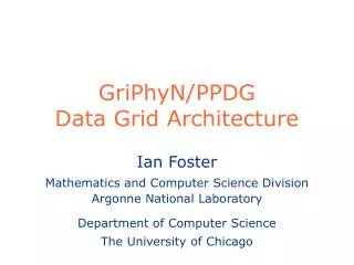
GriPhyN Virtual Data System. Mike Wilde Argonne National Laboratory Mathematics and Computer Science Division LISHEP 2004, UERJ, Rio De Janeiro 13 Feb 2004. A Large Team Effort!. The Chimera Virtual Data System is the work of Ian Foster, Jens Voeckler, Mike Wilde and Yong Zhao

E N D
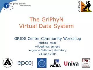
GriPhyN Virtual Data System Mike Wilde Argonne National Laboratory Mathematics and Computer Science Division LISHEP 2004, UERJ, Rio De Janeiro 13 Feb 2004
A Large Team Effort! The Chimera Virtual Data Systemis the work of Ian Foster, Jens Voeckler, Mike Wilde and Yong Zhao The Pegasus Planner is the work of Ewa Deelman, Gaurang Mehta, and Karan Vahi Applications described are the work of many, people, including: James Annis, Rick Cavanaugh, Rob Gardner, Albert Lazzarini, Natalia Maltsev, and their wonderful teams
Acknowledgements GriPhyN, iVDGL, and QuarkNet(in part) are supported by the National Science Foundation The Globus Alliance, PPDG, and QuarkNet are supported in part by the US Department of Energy, Office of Science; by the NASA Information Power Grid program; and by IBM
GriPhyN – Grid Physics Network Mission Enhance scientific productivity through: • Discovery and application of datasets • Enabling use of a worldwide data grid as a scientific workstation Virtual Data enables this approach by creating datasets from workflow “recipes” and recording their provenance.
Virtual Data System Approach Producing data from transformations with uniform, precise data interface descriptions enables… • Discovery: finding and understanding datasets and transformations • Workflow: structured paradigm for organizing, locating, specifying, & producing scientific datasets • Forming new workflow • Building new workflow from existing patterns • Managing change • Planning: automated to make the Grid transparent • Audit: explanation and validation via provenance
psearch –t 10 … file1 file8 simulate –t 10 … file1 file1 File3,4,5 file2 reformat –f fz … file7 conv –I esd –o aod summarize –t 10 … file6 Virtual Data Scenario Manage workflow; Update workflow following changes On-demand data generation Explain provenance, e.g. for file8: • psearch –t 10 –i file3 file4 file5 –o file8summarize –t 10 –i file6 –o file7reformat –f fz –i file2 –o file3 file4 file5 conv –l esd –o aod –i file 2 –o file6simulate –t 10 –o file1 file2
Grid3 – The Laboratory Supported by the National Science Foundation and the Department of Energy.
Virtual Data System Capabilities Producing data from transformations with uniform, precise data interface descriptions enables… • Discovery: finding and understanding datasets and transformations • Workflow: structured paradigm for organizing, locating, specifying, & producing scientific datasets • Forming new workflow • Building new workflow from existing patterns • Managing change • Planning: automated to make the Grid transparent • Audit: explanation and validation via provenance
VDL: Virtual Data LanguageDescribes Data Transformations • Transformation • Abstract template of program invocation • Similar to "function definition" • Derivation • “Function call” to a Transformation • Store past and future: • A record of how data products were generated • A recipe of how data products can be generated • Invocation • Record of a Derivation execution
Example Transformation TR t1( out a2, in a1, none pa = "500", none env = "100000" ) { argument = "-p "${pa}; argument = "-f "${a1}; argument = "-x –y"; argument stdout = ${a2}; profile env.MAXMEM = ${env}; } $a1 t1 $a2
Example Derivations DV d1->t1 (env="20000", pa="600",a2=@{out:run1.exp15.T1932.summary},a1=@{in:run1.exp15.T1932.raw}, ); DV d2->t1 (a1=@{in:run1.exp16.T1918.raw},a2=@{out.run1.exp16.T1918.summary} );
Workflow from File Dependencies file1 TR tr1(in a1, out a2) { argument stdin = ${a1}; argument stdout = ${a2}; } TR tr2(in a1, out a2) { argument stdin = ${a1}; argument stdout = ${a2}; } DV x1->tr1(a1=@{in:file1}, a2=@{out:file2}); DV x2->tr2(a1=@{in:file2}, a2=@{out:file3}); x1 file2 x2 file3
Example Invocation Completion status and resource usage Attributes of executable transformation Attributes of input and output files
Example Workflow • Complex structure • Fan-in • Fan-out • "left" and "right" can run in parallel • Uses input file • Register with RC • Complex file dependencies • Glues workflow preprocess findrange findrange analyze
Workflow step "preprocess" • TR preprocess turns f.a into f.b1 and f.b2 TR preprocess( output b[], input a ) {argument = "-a top";argument = " –i "${input:a};argument = " –o " ${output:b}; } • Makes use of the "list" feature of VDL • Generates 0..N output files. • Number file files depend on the caller.
Workflow step "findrange" • Turns two inputs into one output TR findrange( output b, input a1, input a2,none name="findrange", none p="0.0" ) {argument = "-a "${name};argument = " –i " ${a1} " " ${a2};argument = " –o " ${b};argument = " –p " ${p}; } • Uses the default argument feature
Can also use list[] parameters TR findrange( output b, input a[],none name="findrange", none p="0.0" ) {argument = "-a "${name};argument = " –i " ${" "|a};argument = " –o " ${b};argument = " –p " ${p}; }
Workflow step "analyze" • Combines intermediary results TR analyze( output b, input a[] ) {argument = "-a bottom";argument = " –i " ${a};argument = " –o " ${b}; }
Complete VDL workflow • Generate appropriate derivations DV top->preprocess( b=[ @{out:"f.b1"}, @{ out:"f.b2"} ], a=@{in:"f.a"} ); DV left->findrange( b=@{out:"f.c1"}, a2=@{in:"f.b2"}, a1=@{in:"f.b1"}, name="left", p="0.5" ); DV right->findrange( b=@{out:"f.c2"}, a2=@{in:"f.b2"}, a1=@{in:"f.b1"}, name="right" ); DV bottom->analyze( b=@{out:"f.d"}, a=[ @{in:"f.c1"}, @{in:"f.c2"} );
Compound Transformations • Using compound TR • Permits composition of complex TRs from basic ones • Calls are independent • unless linked through LFN • A Call is effectively an anonymous derivation • Late instantiation at workflow generation time • Permits bundling of repetitive workflows • Model: Function calls nested within a function definition
Compound Transformations (cont) • TR diamond bundles black-diamonds TR diamond( out fd, io fc1, io fc2, io fb1, io fb2, in fa, p1, p2 ) { call preprocess( a=${fa}, b=[ ${out:fb1}, ${out:fb2} ] ); call findrange( a1=${in:fb1}, a2=${in:fb2}, name="LEFT", p=${p1}, b=${out:fc1} ); call findrange( a1=${in:fb1}, a2=${in:fb2}, name="RIGHT", p=${p2}, b=${out:fc2} ); call analyze( a=[ ${in:fc1}, ${in:fc2} ], b=${fd} ); }
Compound Transformations (cont) • Multiple DVs allow easy generator scripts: DV d1->diamond( fd=@{out:"f.00005"}, fc1=@{io:"f.00004"}, fc2=@{io:"f.00003"}, fb1=@{io:"f.00002"}, fb2=@{io:"f.00001"}, fa=@{io:"f.00000"}, p2="100", p1="0" ); DV d2->diamond( fd=@{out:"f.0000B"}, fc1=@{io:"f.0000A"}, fc2=@{io:"f.00009"}, fb1=@{io:"f.00008"}, fb2=@{io:"f.00007"}, fa=@{io:"f.00006"}, p2="141.42135623731", p1="0" ); ... DV d70->diamond( fd=@{out:"f.001A3"}, fc1=@{io:"f.001A2"}, fc2=@{io:"f.001A1"}, fb1=@{io:"f.001A0"}, fb2=@{io:"f.0019F"}, fa=@{io:"f.0019E"}, p2="800", p1="18" );
Virtual Data Example:Galaxy Cluster Search DAG Sloan Data Galaxy cluster size distribution Jim Annis, Steve Kent, Vijay Sehkri, Fermilab, Michael Milligan, Yong Zhao, University of Chicago
Cluster SearchWorkflow Graphand Execution Trace Workflow jobs vs time
mass = 200 decay = bb mass = 200 mass = 200 decay = ZZ mass = 200 decay = WW stability = 3 mass = 200 decay = WW mass = 200 decay = WW stability = 1 mass = 200 event = 8 mass = 200 decay = WW stability = 1 event = 8 mass = 200 plot = 1 mass = 200 decay = WW event = 8 mass = 200 decay = WW stability = 1 plot = 1 mass = 200 decay = WW plot = 1 Virtual Data Application: High Energy Physics Data Analysis mass = 200 decay = WW stability = 1 LowPt = 20 HighPt = 10000 Work and slide by Rick Cavanaugh and Dimitri Bourilkov, University of Florida
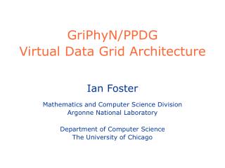
MCAT; GriPhyN catalogs MDS MDS GDMP DAGMAN, Kangaroo GSI, CAS Globus GRAM GridFTP; GRAM; SRM GriPhyN/PPDGData Grid Architecture Application DAG (abstract) Catalog Services Monitoring Planner Info Services DAG (concrete) Repl. Mgmt. Executor Policy/Security Reliable Transfer Service Compute Resource Storage Resource
Job A Job B Job C Job D Executor Example: Condor DAGMan • Directed Acyclic Graph Manager • Specify the dependencies between Condor jobs using DAG data structure • Manage dependencies automatically • (e.g., “Don’t run job “B” until job “A” has completed successfully.”) • Each job is a “node” in DAG • Any number of parent or children nodes • No loops Slide courtesy Miron Livny, U. Wisconsin
DAGMan A Condor Job Queue B B C C D Executor Example: Condor DAGMan (Cont.) • DAGMan acts as a “meta-scheduler” • holds & submits jobs to the Condor queue at the appropriate times based on DAG dependencies • If a job fails, DAGMan continues until it can no longer make progress and then creates a “rescue” file with the current state of the DAG • When failed job is ready to be re-run, the rescue file is used to restore the prior state of the DAG Slide courtesy Miron Livny, U. Wisconsin
Virtual Data in CMS Virtual Data Long Term Vision of CMS: CMS Note 2001/047, GRIPHYN 2001-16
CMS Data Analysis Dominant use of Virtual Data in the Future Event 1 Event 2 Event 3 Tag 2 100b 100b 200b 200b Reconstructed data (produced by physics analysis jobs) Tag 1 Jet finder 2 7K 7K 5K 5K Jet finder 1 Reconstruction Algorithm 100K 100K Calibration data 100K 300K 100K 50K 200K 100K 300K 100K 50K 200K Raw data (simulated or real) 100K 100K 100K 100K 50K 50K Uploaded data Virtual data Algorithms
Production Pipeline GriphyN-CMS Demo pythia cmsim writeHits writeDigis CPU: 2 min 8 hours 5 min 45 min 1 run 1 run 1 run . . . . . . . . . . . . . . . . . . 1 run Data: 0.5 MB 175 MB 275 MB 105 MB truth.ntpl hits.fz hits.DB digis.DB 1 run = 500 events SC2001 Demo Version: 1 event
Pegasus:Planning for Execution in Grids • Maps from abstract to concrete workflow • Algorithmic and AI based techniques • Automatically locates physical locations for both components (transformations and data) • Use Globus Replica Location Service and the Transformation Catalog • find appropriate resources to execute • Via Globus Monitoring and Discovery Serivce • Reuse existing data products where applicable • Publishes newly derived data products • RLS, Chimera virtual data catalog
Computation Replica Location Service • Pegasus uses the RLS to find input data RLI LRC LRC LRC • Pegasus uses the RLS to register new data products
Use of MDS in Pegasus • MDS provides up-to-date Grid state information • Total and idle job queues length on a pool of resources (condor) • Total and available memory on the pool • Disk space on the pools • Number of jobs running on a job manager • Can be used for resource discovery and selection • Developing various task to resource mapping heuristics • Can be used to publish information necessary for replica selection • Developing replica selection components
Job c Job a Job b Job f Job d Job e Job g Job h Job i KEY The original node Input transfer node Registration node Output transfer node Node deleted by Reduction algorithm Abstract Workflow Reduction • The output jobs for the Dag are all the leaf nodes • i.e. f, h, I • Each job requires 2 input files and generates 2 output files. • The user specifies the output location.
KEY The original node Input transfer node Registration node Output transfer node Node deleted by Reduction algorithm Optimizing from the point of view of Virtual Data Job c Job a Job b Job f Job d Job e Job g Job h Job i • Jobs d, e, f have output files that have been found in the Replica Location Service. • Additional jobs are deleted. • All jobs (a, b, c, d, e, f) are removed from the DAG.
KEY The original node Input transfer node Registration node Output transfer node Node deleted by Reduction algorithm Planner picks execution and replica locations Plans for staging data in Job c adding transfer nodes for the input files for the root nodes Job a Job b Job f Job d Job e Job g Job h Job i
transferring the output files of the leaf job (f) to the output location Staging data out and registering new derived products in the RLS Job c Job a Job b Job f Job d Job e Job g Job h Staging and registering for each job that materializes data (g, h, i ). Job i KEY The original node Input transfer node Registration node Output transfer node Node deleted by Reduction algorithm
Input DAG Job g Job h Job c Job a Job b Job i Job f KEY The original node Input transfer node Registration node Output transfer node Job d Job e Job g Job h Job i The final executable DAG
Pegasus Components • Concrete Planner and Submit file generator (gencdag) • The Concrete Planner of the VDS makes the logical to physical mapping of the DAX taking into account the pool where the jobs are to be executed (execution pool) and the final output location (output pool). • Java Replica Location Service Client (rls-client & rls-query-client) • Used to populate and query the globus replica location service.
Pegasus Components (cont’d) • XML Pool Config generator (genpoolconfig) • The Pool Config generator queries the MDS as well as local pool config files to generate a XML pool config which is used by Pegasus. • MDS is preferred for generation pool configuration as it provides a much richer information about the pool including the queue statistics, available memory etc. • The following catalogs are looked up to make the translation • Transformation Catalog (tc.data) • Pool Config File • Replica Location Services • Monitoring and Discovery Services
Transformation Catalog (Demo) • Consists of a simple text file. • Contains Mappings of Logical Transformations to Physical Transformations. • Format of the tc.data file #poolid logical tr physical tr env isi preprocess /usr/vds/bin/preprocess VDS_HOME=/usr/vds/; • All the physical transformations are absolute path names. • Environment string contains all the environment variables required in order for the transformation to run on the execution pool. • DB based TC in testing phase.
Pool Config (Demo) • Pool Config is an XML file which contains information about various pools on which DAGs may execute. • Some of the information contained in the Pool Config file is • Specifies the various job-managers that are available on the pool for the different types of condor universes. • Specifies the GridFtp storage servers associated with each pool. • Specifies the Local Replica Catalogs where data residing in the pool has to be cataloged. • Contains profiles like environment hints which are common site-wide. • Contains the working and storage directories to be used on the pool.
Pool config • Two Ways to construct the Pool Config File. • Monitoring and Discovery Service • Local Pool Config File (Text Based) • Client tool to generate Pool Config File • The tool genpoolconfig is used to query the MDS and/or the local pool config file/s to generate the XML Pool Config file.
Gvds.Pool.Config (Demo) • This file is read by the information provider and published into MDS. • Format gvds.pool.id : <POOL ID> gvds.pool.lrc : <LRC URL> gvds.pool.gridftp : <GSIFTP URL>@<GLOBUS VERSION> gvds.pool.gridftp : gsiftp://sukhna.isi.edu/nfs/asd2/gmehta@2.4.0 gvds.pool.universe : <UNIVERSE>@<JOBMANAGER URL>@< GLOBUS VERSION> gvds.pool.universe : transfer@columbus.isi.edu/jobmanager-fork@2.2.4 gvds.pool.gridlaunch : <Path to Kickstart executable> gvds.pool.workdir : <Path to Working Dir> gvds.pool.profile : <namespace>@<key>@<value> gvds.pool.profile : env@GLOBUS_LOCATION@/smarty/gt2.2.4 gvds.pool.profile : vds@VDS_HOME@/nfs/asd2/gmehta/vds
Properties (Demo) • Properties file define and modify the behavior of Pegasus. • Properties set in the $VDS_HOME/properties can be overridden by defining them either in $HOME/.chimerarc or by giving them on the command line of any executable. • eg. Gendax –Dvds.home=path to vds home…… • Some examples follow but for more details please read the sample.properties file in $VDS_HOME/etc directory. • Basic Required Properties • vds.home : This is auto set by the clients from the environment variable $VDS_HOME • vds.properties : Path to the default properties file • Default : ${vds.home}/etc/properties