Chapter 4 Multiple Regression

1. Chapter 4 Multiple Regression

2. Multiple Regression Overview • What is it? • Why use it?

3. Multiple Regression Y’ = b0 + b1X1 + b2X2 + . . . + bnXn + e Y = Dependent Variable = # of credit cards b0 = intercept (constant) = constant number of credit cards independent of family size and income. b1 = change in credit card usage associated with unit change in family size (regression coefficient). b2 = change in credit card usage associated with unit change in income (regression coefficient). X1 = family size X2 = income e = prediction error (residual)

4. Variate (Y’) = X1b1 + X2b2 + . . . + Xnbn A variate value (Y’) is calculated for each respondent. The Y’ value is a linear combination of the entire set of variables that best achieves the statistical objective. With regression, the variate value is the predicted dependent variable. X3 Y X1 X2

5. Example of a “Business-to-Business” Application of Multiple Regression Performance Measures • Product Quality • Delivery Commitments • Problem Resolution • Competitive Prices • Quality Assurance • Technical Assistance • Creative Pricing / Terms • Technical Alliances • Invoicing • Product Line • Outcome Measures: • Future Purchase • Recommend • Satisfaction

6. What Can We Do With Multiple Regression? • Determine the statistical significance of the attempted prediction. • Determine the strength of association between the single dependent variable and the multiple independent variables. • Identify the relative importance of each of the multiple independent variables in predicting the single metric dependent variable. • Predict the values of the dependent variable from the values of the multiple independent variables.

7. Using Multiple Regression • Sources of variables? • Number of independent variables? • Is More Better ? • Method of variable entry? • Interpretation of regression • functions?

8. Regression Variables? • Sources : • Prior Research ? • Practice – Current Business Situation ? • Theoretical Model ? • Intuition ?

9. Regression Variables ? • Issues : • Measurement Error – Both Dependent & Independents. • Specification Error – Independents only. • Too Few: • lowers prediction. • introduces bias. • Too Many: • Reduces parsimony. • Masks effects of other variables.

10. Variable Selection Approaches: • Confirmatory (Simultaneous). • Sequential Search Methods: • Stepwise (variables not removed once included in regression equation). • Forward Inclusion & Backward Elimination. • Combinatorial (All-Possible-Subsets).

11. Interpretation ofRegression Results: • Coefficient of Determination. • Regression Coefficients (Unstandardized – bivariate). • Beta Coefficients (Standardized). • Variables Entered. • Multicollinearity ??

12. Statistical vs. Practical Significance ? The F statistic is used to determine if the overall regression model is statistically significant. If the F statistic is significant, it means it is unlikely your sample will produce a large R2 when the population R2 is actually zero. To be considered statistically significant, a rule of thumb is there must be <.05 probability the results are due to chance. If the R2 is statistically significant, we then evaluate the strength of the linear association between the dependent variable and the several independent variables. R2, also called the coefficient of determination, is used to measure the strength of the overall relationship. It represents the amount of variation in the dependent variable associated with all of the independent variables considered together (it also is referred to as a measure of the goodness of fit). R2 ranges from 0 to 1.0 and represents the amount of the dependent variable “explained” by the independent variables combined. A large R2 indicates the straight line works well while a small R2 indicates it does not work well. Even though an R2 is statistically significant, it does not mean it is practically significant. We also must ask whether the results are meaningful. For example, is the value of knowing you have explained 4 percent of the variation worth the cost of collecting and analyzing the data?

13. Samouel's Restaurant Description of Employee Survey Variables Variable DescriptionVariable Type Work Environment Measures X1 I am paid fairly for the work I do. Metric X2 I am doing the kind of work I want. Metric X3 My supervisor gives credit an praise for work well done. Metric X4 There is a lot of cooperation among the members of my work group. Metric X5 My job allows me to learn new skills. Metric X6 My supervisor recognizes my potential. Metric X7 My work gives me a sense of accomplishment. Metric X8 My immediate work group functions as a team. Metric X9 My pay reflects the effort I put into doing my work. Metric X10 My supervisor is friendly and helpful. Metric X11 The members of my work group have the skills and/or training to do their job well. Metric X12 The benefits I receive are reasonable. Metric Relationship Measures X13 Loyalty – I have a sense of loyalty to Samouel’s restaurant. Metric X14 Effort – I am willing to put in a great deal of effort beyond that expected to help Samouel’s restaurant to be successful. Metric X15 Proud – I am proud to tell others that I work for Samouel’s restaurant. Metric Classification Variables X16 Intention to Search Metric X17 Length of Time an Employee Nonmetric X18 Work Type = Part-Time vs. Full-Time Nonmetric X19 Gender Nonmetric X20 Age Nonmetric X21 Performance Metric

14. Description of Customer Survey Variables GINO'S Samouel's Restaurant VS. Variable DescriptionVariable Type Restaurant Perceptions X1 Excellent Food Quality Metric X2 Attractive Interior Metric X3 Generous Portions Metric X4 Excellent Food Taste Metric X5 Good Value for the Money Metric X6 Friendly Employees Metric X7 Appears Clean & Neat Metric X8 Fun Place to Go Metric X9 Wide Variety of menu Items Metric X10 Reasonable Prices Metric X11 Courteous Employees Metric X12 Competent Employees Metric Selection Factor Rankings X13 Food Quality Nonmetric X14 Atmosphere Nonmetric X15 Prices Nonmetric X16 Employees Nonmetric Relationship Variables X17 Satisfaction Metric X18 Likely to Return in Future Metric X19 Recommend to Friend Metric X20 Frequency of Patronage Nonmetric X21 Length of Time a Customer Nonmetric Classification Variables X22 Gender Nonmetric X23 Age Nonmetric X24 Income Nonmetric X25 Competitor Nonmetric X26 Which AD Viewed (#1, 2 or 3) Nonmetric X27 AD Rating Metric X28 Respondents that Viewed Ads Nonmetric

15. Selected Variables from Samouel’s Customer Survey X1 – Excellent Food Quality Strongly Strongly Disagree Agree 1 2 3 4 5 6 7 X4 – Excellent Food Taste Strongly Strongly Disagree Agree 1 2 3 4 5 6 7 X9 – Wide Variety of Menu Items Strongly Strongly Disagree Agree 1 2 3 4 5 6 7 X18 – How likely are you to return to Samouel’s restaurant in the future? Definitely Will Definitely Will Not Return Return 1 2 3 4 5 6 7

16. Using SPSS to Compute a Multiple Regression Model: We want to compare Samouel’s customers’ perceptions with those of Gino’s, so go to the Data pull-down menu to split the sample. Scroll down and click on Split File, then on Compare Groups. Highlight variable X25 and move it into the box labeled “Groups based on:” and then click OK. Now you can run the regression and compare Samouel’s and Gino’s. The SPSS click through sequence is ANALYZE  REGRESSION  LINEAR. Highlight X18 and move it to the dependent variables box. Highlight X1, X4 and X9 and move them to the independent variables box. Use the default “Enter” in the Methods box. Click on the Statistics button and use the defaults for “Estimates” and “Model Fit”. Next click on “Descriptives” and then Continue. There are several other options you could select at the bottom of this dialog box but for now we will use the program defaults. Click on “OK” at the top right of the dialog box to run the regression. To run stepwise multiple regression, follow the same procedure as described above except go to the “Methods” box and where it has “Enter” as the default click on the arrow box and go to “Stepwise” and click on it. Then click on “OK” at the top right of the dialog box to run the stepwise regression.

17. Multiple Regression Dialog Boxes

18. Multiple Regression Output Adjusted R-Square = reduces the R2 by taking into account the sample size and the number of independent variables in the regression model (It becomes smaller as we have fewer observations per independent variable). R-Square = the amount of variation in Y explained by the X’s. Standard Error of the Estimate (SEE) = a measure of the accuracy of the regression predictions. It estimates the variation of the dependent variable values around the regression line. It should get smaller as we add more independent variables, if they predict well.

19. Multiple Regression Output continued . . . Degrees of freedom (df)  = the total number of observations minus the number of estimated parameters. For example, in estimating a regression model with a single independent variable, we estimate two parameters, the intercept (b0) and a regression coefficient for the independent variable (b1). If the number of degrees of freedom is small, the resulting prediction is less generalizable. Conversely, a large degrees-of-freedom value indicates the prediction is fairly “robust” with regard to being representative of the overall sample of respondents. Total Sum of Squares (SST) = total amount of variation that exists to be explained by the independent variables. TSS = the sum of SSE and SSR. Sum of Squares Regression (SSR) = the amount of improvement in explanation of the dependent variable attributable to the independent variables. Sum of Squared Errors (SSE) = the variance in the dependent variable not accounted for by the regression model = residual. The objective is to obtain the smallest possible sum of squared errors as a measure of prediction accuracy.

20. Multiple Regression Output continued . . . Beta interpretation = for every unit the Samouel’s X1 beta increases, X18 (dependent variable) will increase by .324 units. Only significant betas are interpreted (=/> .05). Constant term (b0) = also referred to as the intercept, it is the value on the Y axis (dependent variable axis) where the line defined by the regression equation crosses the axis.

21. Multiple RegressionLearning Checkpoint When should multiple regression be used? Why should multiple regression be used? What level of statistical significance and R2 would justify use of multiple regression? How do you use regression coefficients?

22. Advanced Topics in Multiple Regression • Multicollinearity • Dummy Variables • Assumptions

23. . . . . is the correlation among the independent variables. Multicollinearity

24. Multicollinearity Diagnostics: • Variance Inflation Factor (VIF) – measures how much the variance of the regression coefficients is inflated by multicollinearity problems. If VIF equals 0, there is no correlation between the independent measures. A VIF measure of 1 is an indication of some association between predictor variables, but generally not enough to cause problems. A maximum acceptable VIF value would be 5.0; anything higher would indicate a problem with multicollinearity. • Tolerance – the amount of variance in an independent variable that is not explained by the other independent variables. If the other variables explain a lot of the variance of a particular independent variable we have a problem with multicollinearity. Thus, small values for tolerance indicate problems of multicollinearity. The minimum cutoff value for tolerance is typically .20. That is, the tolerance value must be smaller than .20 to indicate a problem of multicollinearity.

25. Using SPSS to Examine Multicollinearity: The SPSS click through sequence is: ANALYZE  REGRESSION  LINEAR. Go to Samouel’s employee survey data and click on X13 – Loyalty and move it to the Dependent Variables box. Click on variables X1 to X12 and move them to the Independent Variables box. The box labeled “Method” has ENTER as the default and we will use it. Click on the “Statistics” button and use the “Estimates” and “Model fit” defaults. Click on “Descriptives” and “Collinearity diagnostics” and then “Continue” and “OK” to run the regression.

26. Dummy Variable • . . . . a nonmetric independent variable that has two (or more) distinct levels, that are coded 0 and 1.

27. Selected Variables from Employee Survey Independent Variables (Job Satisfaction & Gender) 2. I am doing the kind of work I want. Strongly Strongly Disagree Agree 1 2 3 4 5 6 7 5. My job allows me to learn new skills. Strongly Strongly Disagree Agree 1 2 3 4 5 6 7 7. My work give me a sense of accomplishment. Strongly Strongly Disagree Agree 1 2 3 4 5 6 7 19. Gender 0 = Male 1 = Female Dependent Variable 15. I am proud to tell others that I work for Samouel’s restaurant. Strongly Strongly Disagree Agree 1 2 3 4 5 6 7

28. Using SPSS to Examine Dummy Variables: The SPSS click through sequence is: ANALYZE  REGRESSION  LINEAR. Go to Samouel’s employee survey data and click on X15 – Proud and move it to the Dependent Variables box. Click on X2, X5, X7 and X19 and move them to the Independent Variables box. The box labeled “Method” has ENTER as the default and we will use it. Click on the “Statistics” button and use the “Estimates” and “Model fit” defaults. Click on “Descriptives” then “Continue” and “OK” to run the regression.

29. Multiple Regression Assumptions: • Metrically measured variables. • Linearity. • Minimal multicollinearity among independent variables. • Constant variance of error terms (residuals). • Independence of error terms. • Normality of error term distribution.

30. Regression Analysis Terms • Explained variance = R2 (coefficient of determination). • Unexplained variance = residuals (error).

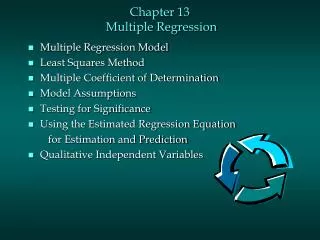
31. Least Squares Regression Line Y Deviation not explained by regression Total Deviation Y = average Deviation explained by regression X

32. Residuals Plots • Histogram of standardized residuals – enables you to determine if the errors are normally distributed (see Exhibit 1; also Hair pp. 174-5). • Normal probability plot – enables you to determine if the errors are normally distributed. It compares the observed (sample) standardized residuals against the expected standardized residuals from a normal distribution (see Exhibit 2). • ScatterPlot of residuals – can be used to test regression assumptions. It compares the standardized predicted values of the dependent variable against the standardized residuals from the regression equation (see Exhibit 3). If the plot exhibits a random pattern then this indicates no identifiable violations of the assumptions underlying regression analysis.

33. Exhibit 1: Histogram of Employee Survey Dependent Variable X15 – Proud

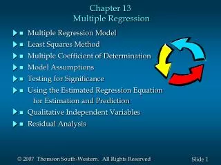
34. Exhibit 2: Normal Probability Plot of Regression Standardized Residuals Normal probability plot = a graphical comparison of the shape of the sample distribution (observed) to the normal distribution. The straight line angled at 45 degrees is the normal distribution and the actual distribution (observed) is shown as deviations from the straight line.

35. Exhibit 3: Scatterplot of Employee Survey Dependent Variable X15 – Proud This is a scatterplot of the standardized residuals versus the predicted dependent (Y) values. If it exhibits a random pattern, which this plot does, then it indicates no identifiable violations of the assumptions underlying regression analysis and is called a “Null Plot”. See Hair, pp. 173-174.

36. Using SPSS to Examine Residuals: SPSS includes several diagnostic tools to examine residuals. To run the regression that examines the residuals, first load the employee database. The click through sequence is ANALYZE  REGRESSION  LINEAR. Highlight X15 – Proud and move it to the dependent variable box. Next highlight variables X2, X5, X7, and X19 and move them to the independent variable box. ‘Enter’ is the default in the Methods box and we will use it. Click on the Statistics button and ‘Estimates’ and ‘Model Fit’ will be the defaults (if they are not defaults in your version of SPSS click them). Now, click on ‘Collinearity Diagnostics’ and then go to the bottom left of the screen in the Residuals box and click on ‘Casewise Diagnostics’. The default is to identify outliers outside 3 standard deviations, but in this case we are going to be conservative and use 2 standard deviations. Click on Outliers outside and then place a 2 in the box for number of standard deviations. Next click on Continue. This is the same sequence as earlier regression applications, but now we also must go to the Plots button to request some new information. To produce plots of the residuals to check on potential violations of the regression assumptions, click on “ZPRED” and move it to the “Y” box. Then click on “ZRESID” and move it to the “X” box. These two plots are for the Standardized Predicted Dependent Variable and Standardized Residuals. Next, click on Histogram and Normal Probability plot under the Standardized Residual Plots box on the lower left side of the screen. Examination of these plots and tables enables us to determine whether the hypothesized relationship between the dependent variable X15 and the independent variables X2, X5, X7, and X19 is linear, and also whether the error terms in the regression model are normally distributed. Finally, click on ‘Continue’ and then on ‘OK’ to run the program. The results are the same as in Exhibits 1 to 3.

37. DESCRIPTION OF DATABASE VARIABLES Variable Description Variable Type PERCEPTIONS OF HATCO X1 Delivery speed Metric X2 Price level Metric X3 Price flexibility Metric X4 Manufacturer’s image Metric X5 Overall service Metric X6 Salesforce image Metric X7 Product quality Metric PURCHASE OUTCOMES X9 Usage level Metric X10 Satisfaction level Metric PURCHASER CHARACTERISTICS X8 Size of firm Nonmetric X11 Specification buying Nonmetric X12 Structure of procurement Nonmetric X13 Type of industry Nonmetric X14 Type of buying situation Nonmetric

38. Samouel's Restaurant Description of Employee Survey Variables Variable DescriptionVariable Type Work Environment Measures X1 I am paid fairly for the work I do. Metric X2 I am doing the kind of work I want. Metric X3 My supervisor gives credit an praise for work well done. Metric X4 There is a lot of cooperation among the members of my work group. Metric X5 My job allows me to learn new skills. Metric X6 My supervisor recognizes my potential. Metric X7 My work gives me a sense of accomplishment. Metric X8 My immediate work group functions as a team. Metric X9 My pay reflects the effort I put into doing my work. Metric X10 My supervisor is friendly and helpful. Metric X11 The members of my work group have the skills and/or training to do their job well. Metric X12 The benefits I receive are reasonable. Metric Relationship Measures X13 Loyalty – I have a sense of loyalty to Samouel’s restaurant. Metric X14 Effort – I am willing to put in a great deal of effort beyond that expected to help Samouel’s restaurant to be successful. Metric X15 Proud – I am proud to tell others that I work for Samouel’s restaurant. Metric Classification Variables X16 Intention to Search Metric X17 Length of Time an Employee Nonmetric X18 Work Type = Part-Time vs. Full-Time Nonmetric X19 Gender Nonmetric X20 Age Nonmetric X21 Performance Metric

39. Description of Customer Survey Variables GINO'S Samouel's Restaurant VS. Variable DescriptionVariable Type Restaurant Perceptions X1 Excellent Food Quality Metric X2 Attractive Interior Metric X3 Generous Portions Metric X4 Excellent Food Taste Metric X5 Good Value for the Money Metric X6 Friendly Employees Metric X7 Appears Clean & Neat Metric X8 Fun Place to Go Metric X9 Wide Variety of menu Items Metric X10 Reasonable Prices Metric X11 Courteous Employees Metric X12 Competent Employees Metric Selection Factor Rankings X13 Food Quality Nonmetric X14 Atmosphere Nonmetric X15 Prices Nonmetric X16 Employees Nonmetric Relationship Variables X17 Satisfaction Metric X18 Likely to Return in Future Metric X19 Recommend to Friend Metric X20 Frequency of Patronage Nonmetric X21 Length of Time a Customer Nonmetric Classification Variables X22 Gender Nonmetric X23 Age Nonmetric X24 Income Nonmetric X25 Competitor Nonmetric X26 Which AD Viewed (#1, 2 or 3) Nonmetric X27 AD Rating Metric X28 Respondents that Viewed Ads Nonmetric