Download

1 / 20
200 likes | 305 Views
Sequence comparison: Score matrices. http://faculty.washington.edu/jht/GS559_2012/. Genome 559: Introduction to Statistical and Computational Genomics Prof. James H. Thomas. FYI - informal inductive proof of best alignment path.

E N D
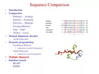
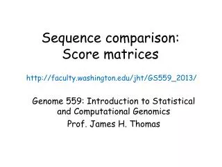
Sequence comparison: Score matrices http://faculty.washington.edu/jht/GS559_2012/ Genome 559: Introduction to Statistical and Computational Genomics Prof. James H. Thomas
FYI - informal inductive proof of best alignment path Consider the last step in the best alignment path to node abelow. This path must come from one of the three nodes shown, where X, Y, and Z are the cumulative scores of the best alignments up to those nodes. We can reach node a by three possible paths: an A-B match, a gap in sequence A or a gap in sequence B: The best-scoring path to a is the maximum of: X + match Y + gap Z + gap BUT the best paths to X, Y, and Z are analogously the max of their three upstream possibilities, etc. Inductively QED.
Local alignment - review d = -5 2 0 (no arrow means no preceding alignment)
Two differences from global alignment: If a score is negative, replace with 0. Traceback from the highest score in the matrix and continue until you reach 0. Global alignment algorithm: Needleman-Wunsch. Local alignment algorithm: Smith-Waterman. Local alignment
dot plot of two DNA sequences overlay of the global DP alignment path
Protein score matrices • Quantitatively represent the degree of conservation of typical amino acid residues over evolutionary time. • All possible amino acid changes are represented (matrix of size at least 20 x 20). • Most commonly used are several different BLOSUM matrices derived for different degrees of evolutionary divergence. • DNA score matrices are simpler (and conceptually similar).
BLOSUM62 Score Matrix regular 20 amino acids # BLOSUM Clustered Scoring Matrix in 1/2 Bit Units # Cluster Percentage: >= 62 ambiguity codes and stop
Amino acid structures Hydrophobic Polar Charged phenylalanine F
BLOSUM62 Score Matrix Good scores – chemically similar Bad scores – chemically dissimilar
Amino acid structures Hydrophobic Polar Charged
Deriving BLOSUM scores • Find sets of sequences whose alignment is thought to be correct (this is partly bootstrapped by alignment). • Measure how often various amino acid pairs occur in the alignments. • Normalize this to the expected frequency of such pairs randomly in the same set of alignments. • Derive a log-odds score for aligned vs. random.
Example of alignment block (the BLO part of BLOSUM) 31 positions (columns) 61 sequences (rows) • Thousands of such blocks go into computing a single BLOSUM matrix. • Represent full diversity of sequences. • Results are summed over all columns of all blocks.
Pair frequency vs. expectation Sample column from an alignment block: Actual aligned pair frequency: this is called the sum of pairs (the SUM part of BLOSUM) D E D N D D etc. 6 D-D pairs 4 D-E pairs 4 D-N pairs 1 E-N pair Randomly expected pair frequency: (a multiple alignment of N sequences is the equivalent of all the pairwise alignments, which number (N)(N-1)/2.)
Log-odds score calculation (so adding scores == multiplying probabilities) For computational speed often rounded to nearest integer and (to reduce round-off error) they are often multiplied by 2 (or more) first, giving a “half-bit” score: (computers can add integers faster than floats)
BLOSUM62 matrix (half-bit scores) ( 9 half-bits = 4.5 bits ) Frequency of C residue over all proteins: 0.0162 (you have to look this up) Reverse calculation of aligned C-C pair frequency in BLOSUM data set: C-C thus
Constructing Blocks • Blocks are ungapped alignments of multiple sequences, usually 20 to 100 amino acids long. • Cluster the members of each block according to their percent identity. • Make pair counts and score matrix from a large collection of similarly clustered blocks. • Each BLOSUM matrix is named for the percent identity cutoff in step 2 (e.g. BLOSUM70 for 70% identity).
this alignment has a score of 16 (6+2+1+7) by BLOSUM 62, meaning an alignment with this score or more is 28(256) times more likely than expected from a random alignment. FIAP FLSP • this 15 amino acid alignment has a score of 75, meaning that it is ~1011 times more likely to be seen in a real alignment than in a random alignment(!!). VHRDLKPENLLLASK VHRDLKPENLLLASK (4+8+5+6+4+5+7+5+6+4+4+4+4+4+5) Probabilistic Interpretation of Scores (ungapped) (BLOSUM62) • By converting scores back to probabilities, we can give a probabilistic interpretation to an alignment score.
Randomly Distributed Gaps (probability of a gap at each position in the sequence) if then [note - the slope of the line on a log-linear plot will vary according to the frequency of gaps, but it will always be linear]
Distribution of real alignment gap lengths in large set of structurally-aligned proteins log-linear plot Nowhere near linear - hence the use of affine gap penalties (there ideally would be several levels of decreasing affine penalties)
What you should know • How a score matrix is derived • What the scores mean probablistically • Why gap penalties should be affine