An Experimental Study of Spatial Variability of Rainfall:

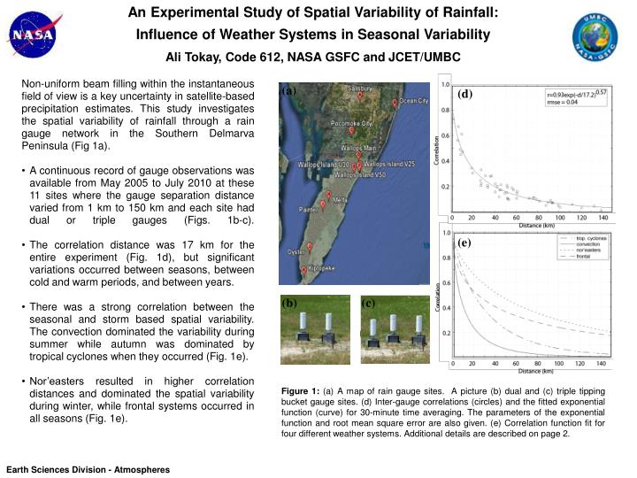
1. An Experimental Study of Spatial Variability of Rainfall: Influence of Weather Systems in Seasonal VariabilityAli Tokay, Code 612, NASA GSFC and JCET/UMBC • Non-uniform beam filling within the instantaneous field of view is a key uncertainty in satellite-based precipitation estimates. This study investigates the spatial variability of rainfall through a rain gauge network in the Southern Delmarva Peninsula (Fig 1a). • A continuous record of gauge observations was available from May 2005 to July 2010 at these 11 sites where the gauge separation distance varied from 1 km to 150 km and each site had dual or triple gauges (Figs. 1b-c). • The correlation distance was 17 km for the entire experiment (Fig. 1d), but significant variations occurred between seasons, between cold and warm periods, and between years. • There was a strong correlation between the seasonal and storm based spatial variability. The convection dominated the variability during summer while autumn was dominated by tropical cyclones when they occurred (Fig. 1e). • Nor’easters resulted in higher correlation distances and dominated the spatial variability during winter, while frontal systems occurred in all seasons (Fig. 1e). (a) (d) (e) (b) (c) Figure 1:(a) A map of rain gauge sites. A picture (b) dual and (c) triple tipping bucket gauge sites. (d) Inter-gauge correlations (circles) and the fitted exponential function (curve) for 30-minute time averaging. The parameters of the exponential function and root mean square error are also given. (e) Correlation function fit for four different weather systems.Additional details are described on page 2. Earth Sciences Division - Atmospheres

2. Name: Ali Tokay, NASA/GSFC, Code 612 and JCET/UMBC E-mail: ali.tokay-1@nasa.gov Phone: 301-614-6140 Reference: Tokay, A., R. J. Roche, and P. G. Bashor, 2014: An experimental study of spatial variability of rainfall. J. Hydrometeorology, 15m 810-812. doi:10.1175/JHM-D-13-031.1 Contributors: Rigoberto J. Roche (FIU, NASA/GSFC Summer Intern), Paul G. Bashor (NASA/GSFC/WFF) Data Sources: Rain gauge data from Southern Delmarva Peninsula. Technical Description of Figures: Figure 1: (a) A map of rain gauge sites in the Southern Delmarva Peninsula. A total of 30 tipping bucket gauges collected over 18000 rainy 5-minute samples. (b) A picture of dual and (c) triple tipping bucket gauge sites. (d) Inter-gauge correlations (circles) and the fitted exponential function (curve) for 30-minute time averaging. The parameters of the exponential function and root mean square error are also given. The correlation distance is not only function of precipitation characteristics but also depends on the distribution of gauges, rain/no-rain threshold, and integration period. (e) Correlation of function fit for four different weather systems. The correlations were lower in convection, while nor’easters resulted in higher correlation at a given distance. There were similarities in correlation distances between summer (not shown) and convection as well as between winter (not shown) and nor’easters. Scientific significance: This study intends to quantify the spatial variability of rainfall within the instantaneous field of view of microwave-sensor-based rainfall estimates and within the footprint of spaceborne radars. The dominance of particular weather systems in a given season and warm/cold period is one of the key conclusions of this study. The unique database with continuous gauge record over 5 years enabled the investigation of the spatial variability between the years in a given season, warm/cold periods, and year. Interestingly, the spatial variability was noticeably different between the years in the presence and absence of topical cyclones during autumn. Relevance for future science and relationship to Decadal Survey: The study was conducted under the NASA Global Precipitation Measurement (GPM) mission ground validation program. The study showed the importance of long-term collection of precipitation data. While the two-month-long field campaigns (e.g. Mid-latitude Continental Convective Clouds Experiment) aims to answer several key questions of the spaceborne algorithm developers, the long-term data collection from direct observations sites enabled the study of seasonal and longer term variability of precipitation. Earth Sciences Division - Atmospheres

3. Accounting for snow darkening over land surface in NASA’s GEOS-5 Model Teppei J. Yasunari (Code 613; GESTAR/USRA) and K.-M. Lau (Code 610; NASA)at NASA GSFC • Dust, black carbon (BC), and organic carbon (OC) depositions on snow can reduce its reflectance (albedo), possibly accelerating snow melting (called, snow darkening effect: SDE; see the references in Yasunari et al., 2014). Understanding the feedbacks between land and atmosphere due to the SDE is one of the important topics in climate science. • Yasunari et al. (2014)summarized the developed GOddardSnoWImpurity Module (GOSWIM)implemented in NASA GSFC’s system for Earth System Modeling (called GEOS-5) to account for dust, BC, and OC SDE over the land surface. • With a 1-D off-line simulation at Sapporo (Japan), reasonable seasonal migrations of snow-covered surface albedos and snow depth were simulated by the Catchment land surface model (LSM) for GEOS-5 Model with GOSWIM with the forcing data (see the next page) (Exp 1; Figure 1) • However, dust and BC in the snow surface were underestimated except for the BC in the early winter (Figure 2). This could be explained by the underestimates of dust and BC depositions with another sensitivity off-line simulation, increasing these depositions (Exp 2). • Another sensitivity off-line simulation with zero BC depositions (Exp 2-2) under the meteorologicaland aerosol conditions of Exp 2, expecting a BC-free urban city, suggested that the duration of snowcover in Sapporo could be prolonged by as much as four days without BC depositions. • With the implementation of GOSWIM, NASA’s GEOS-5 is now ready for global SDE simulations over the land surface (see the next page too). Figure 1: An one-winter 1-D off-line simulation with GOSWIM/Catchment LSM (2007/2008) at Sapporo (Japan) for visible (line in red) and near infrared (line in blue) surface albedos, and snow depth (pink), compared to observations (surface albedos: points in the same colors as the simulated ones; snow depth: black and green lines by JMA and by Aoki et al. 2011, respectively). Vertical lines in turquoise and gray indicate the timing of the inferred rainfall and snowfall with the JMA observations. This simulation is the baseline experiment (Exp 1). Figure 2: Simulated (Exp 1; lines; the top snow layer; maximum of 0.08 m) and observed (points; Aoki et al., 2011; top 10 cm of snow) mass concentrations of dust (blue), BC (black), and OC (red) in the snow surface. The vertical lines are the same as those of Figure 1. The vertical axis is in log scale. Earth Sciences Division - Atmospheres Just remember as “Let’s GOSWIM with GOCART in NASA GEOS-5!”

4. Name: Teppei J. Yasunari, NASA/GSFC, Code 613 and GESTAR/USRAE-mail: teppei.j.yasunari@nasa.gov Phone: 301-614-6199 References: Aoki, T., K. Kuchiki, M. Niwano, Y. Kodama, M. Hosaka, and T. Tanaka (2011), Physically based snow albedo model for calculating broadband albedos and the solar heating profile in snowpack for general circulation models, J. Geophys. Res., 116, D11114, doi:10.1029/2010JD015507. Yasunari, T. J., R. D. Koster, K.-M. Lau, T. Aoki, Y. C. Sud, T. Yamazaki, H. Motoyoshi, and Y. Kodama (2011), Influence of dust and black carbon on the snow albedo in the NASA Goddard Earth Observing System version 5 land surface model, J. Geophys. Res., 116, D02210, doi:10.1029/2010JD014861. Yasunari, T. J., K.-M. Lau, S. P. P. Mahanama, P. R. Colarco, A. M. da Silva, T. Aoki, K. Aoki, N. Murao, S. Yamagata, and Y. Kodama (2014), The GOddardSnoW Impurity Module (GOSWIM) for the NASA GEOS-5 Earth System Model: Preliminary comparisons with observations in Sapporo, Japan, SOLA, 10, 50−56, doi:10.2151/sola.2014-011. (Available with open access at: https://www.jstage.jst.go.jp/article/sola/10/0/10_2014-011/_article). Data Sources: The observed mass concentrations of dust, BC, and OC in snow, surface albedos calculated from incoming and upwelling radiations, and snow depth at Institute of Low Temperature Science in Hokkaido University (ILTS; Sapporo, Japan) were used from Aoki et al. (2011). The meteorological and snow depth data at Sapporo were observed and maintained by the Japan Meteorological Agency (JMA), and these were obtained from its website (available in Japanese at: http://www.data.jma.go.jp/obd/stats/etrn/index.php). The JMA-based meteorological data (estimates were included) and GOCART aerosol depositions at Sapporo from a global GEOS-5 simulation were used for the off-line simulations as the forcing data (Yasunari et al., 2014). Technical Description of Figures (figures and its captions are from and based on Yasunari et al., 2014, respectively) : Figure 1: An one-winter 1-D off-line simulation with GOSWIM/Catchment LSM (2007/2008) at Sapporo (Japan) for visible (line in red) and near infrared (line in blue) surface albedos (vegetation and snow), and snow depth (pink), compared to observations (surface albedos: points in the same colors as the simulated ones; snow depth: black and green lines by JMA and by Aoki et al. 2011, respectively). Vertical lines in turquoise and gray indicate the timing of the inferred rainfall and snowfall with the JMA observations. This simulation is the baseline experiment (Exp1). At the timing of the proofreading, a formulation error was found in GOSWIM, but this could generate negligible errors at Sapporo based on the repeated some 1-D off-line simulations with the correction (mentioned in the Supplemental Information of Yasunari et al., 2014). See more details on the simulation settings in Yasunari et al. (2014). Figure 2: Simulated (Exp 1; lines; the top snow layer; maximum of 0.08 m) and observed (points; Aoki et al., 2011; top 10 cm of snow) mass concentrations of dust (blue), BC (black), and OC (red) in the snow surface. The vertical lines are the same as those of Figure 1. The vertical axis is in log scale. Scientific significance: Before the development of GOSWIM, there was no way to calculate SDE using the Light Absorbing Aerosol (LAA) depositions from the chemical transport module, GOCART, in NASA’s GEOS-5. The development of SDE components started from the preliminary incorporation of dust and BC SDE on the snow albedo calculation in the Catchment LSM for off-line simulations (Yasunari et al., 2011), and extended to the recent updates of the snow albedo components and the new addition of the mass concentration scheme by Yasunari et al. (2014). Then, we named the snow darkening components for GEOS-5 as GOSWIM. NASA GEOS-5 is now equipped to globally simulate the SDE by dust, BC, and OC (i.e., LAA) depositions from the atmosphere over the snow at the model defined land surface tiles in the Catchment LSM (currently excluding the land ice such as glaciers and the ice sheets, and sea ice parts). Thus capability allows GEOS-5 to simulate climate feedbacks between the land surface and atmosphere caused by SDE. Relevance to future science and NASA missions: Taking into account the effect of snow impurities (i.e., LAA) in surface albedo calculations is an important task to be undertaken by the global modeling community in its effort to assess climate impacts of LAA pollutions. NASA GEOS-5 is on its way to improve its capabilities in that regard. We would like to emphasize that without process-oriented observations on SDE in the future, further GOSWIM improvements are very difficult because still we have limited knowledge on the SDE-related processes so far as summarized in Yasunari et al. (2014). Therefore, many in-situ and satellite observations together with model developments on the processes are encouraged in the future to reduce the uncertainties on SDE in global climate model simulations. At the same time our studies imply that there is need for spectrally resolved observations of surface reflectance and this requirement should therefore receive serious consideration during the development of future space-based NASA Earth-observing systems. Modeling supports by NASA would also be essential to implement better forecasting, future climate predictions, and others. Earth Sciences Division - Atmospheres

5. Destruction of Mesospheric Ozone Caused by Solar Protons in March 2012 Charles Jackman (Code 614, NASA GSFC) and Eric Fleming (SSAI and Code 614, NASA GSFC) EOS Aura Solar eruptions in 2012 led to a substantial barrage of charged particles on the Earth’s polar atmosphere during the March 7-11 period. Most of these charged particles were protons, thus the term “Solar Proton Event (SPE)” has been used to describe this phenomenon. The solar protons created hydrogen-containing compounds, which led to the polar ozone destruction. We have used the Aura Microwave Limb Sounder (MLS) observations and a global model simulation to quantify the changes in ozone due to this SPE. The MLS measured atmospheric changes in ozone for the latitude bands 60-82.5oN and 60-82.5oS shown in Figure 1 (top) are all relative to the quiet March 2-6, 2012 time period, which contained no SPEs. Predicted results from the Goddard Space Flight Center (GSFC) two-dimensional (2-D) model are shown in Figure 1 (bottom).The SPE-caused mesospheric and upper stratospheric ozone decreases (up to 80% in the 60-82.5oN band and over 40% in the 60-82.5oS band) are indicated in the Figure. The ozone changes at pressure levels >2 hPa in the 60-82.5oN band, below the large ozone decreases, are mostly seasonal variations, not connected to the SPEs. March 2012 March 2012 Figure 1. Daily averaged ozone changes from Aura MLS measurements (Top) and GSFC 2-D model predictions (Bottom) for the 60-82.5oN band (left plots) and for the 60-82.5oS band (right plots). An average observed (predicted) ozone profile for the period March 2-6, 2012 was subtracted from the observed (predicted) ozone values for the plotted days of March 6-11, 2012 for Aura measurements (Top) and GSFC 2-D model simulation “B(with SPEs)”. The MLS averaging kernel (AK) was used to sample the model results. The contour intervals for the ozone differences are -80, -60, -40, -20, -10, -5, -2, -1, 0, 1,2,5, and 10%). Earth Sciences Division - Atmospheres

6. Name: Charles Jackman, NASA/GSFC, Code 614 E-mail: Charles.H.Jackman@nasa.gov Phone: 301-614-6053 Reference: Jackman, C. H., C. E. Randall, V. L. Harvey, S. Wang, E. L. Fleming, M. Lopez-Puertas, B. Funke, and P. F. Bernath, Middle atmospheric changes caused by the January and March 2012 solar proton events, Atmos. Chem. Phys., 14, 1025-1038, 2014. Data Sources: NASA EOS Aura Microwave Limb Sounder (MLS) v2 data Technical Description of Figure: We adapt Figure 5 of Jackman et al. (2014) to be able to compare MLS-measured ozone in the same Figure. This Figure shows the Solar Proton Event caused changes in the upper stratosphere and mesosphere in the polar regions (60-82.5oN and 60-82.5oS) in the period March 6-11, 2012. Scientific significance: Variations in ozone have been caused by both natural and humankind related processes. The humankind or anthropogenic influence on ozone originates from the chlorofluorocarbons and halons (chlorine and bromine) and has led to international regulations greatly limiting the release of these substances. Certain natural ozone influences are also important in polar regions and are caused by the impact of solar charged particles on the atmosphere. Such natural variations have been studied in order to better quantify the human influence on polar ozone. The Solar Proton Event (SPE) of March 2012 caused huge measured polar enhancements in the HOx (H, OH, HO2) and NOx (N, NO, NO2) constituents, which led to the destruction of mesospheric and upper stratospheric ozone. Simulations with the Goddard Space Flight Center (GSFC) two-dimensional (2-D) model of the changes in HO2 and ozone in March 2012 are similar to the Aura MLS measured changes, however, the predictions of the HO2 enhancements are slightly higher (not shown) indicating that there may be a small problem in the modeled representation of the HOx chemistry. These SPEs also produced longer-lived NOx constituents (not shown), which lasted over a month past their initial production by the solar protons. The SPE-produced NOx constituents were simulated with the GSFC 2-D model as well as the Global Modeling Initiative (GMI) three-dimensional (3-D) chemistry and transport model (CTM). The NOx constituents were transported away from their production region and caused a longer lasting ozone change in the middle to upper stratosphere. Although SPEs are sporadic, they mostly occur near solar maximum. SPEs cause a prompt, predictable perturbation to the atmosphere and can be used to test the chemistry and transport in global models. SPEs, also, can influence the polar regions where their impact on ozone needs to be measured and better predicted so that humankind-caused ozone variations can be more reliably quantified. Relevance for future science and relationship to Decadal Survey: This work shows the importance of solar-related processes in the observed variation of the atmosphere. It will be important to carry out further measurements of HOx and NOx constituents as well as ozone in order to understand the variations in middle atmospheric gases. Thus, measurements of the proposed Decadal Survey’s Global Atmospheric Composition Mission (GACM) are necessary to continue the work on the influence of solar protons on the mesosphere and stratosphere. EOS Aura Earth Sciences Division - Atmospheres