Download
1 / 31
310 likes | 441 Views
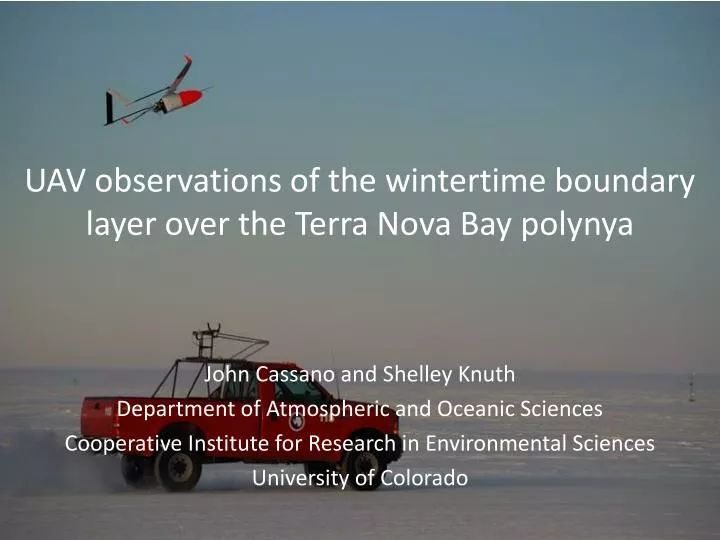
UAV observations of the wintertime boundary layer over the Terra Nova Bay polynya. John Cassano and Shelley Knuth Department of Atmospheric and Oceanic Sciences Cooperative Institute for Research in Environmental Sciences University of Colorado. Project Overview.

E N D
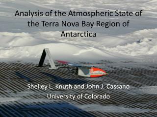
UAV observations of the wintertime boundary layer over the Terra Nova Bay polynya John Cassano and Shelley Knuth Department of Atmospheric and Oceanic Sciences Cooperative Institute for Research in Environmental Sciences University of Colorado
Project Overview • Use Aerosonde unmanned aerial vehicles (UAVs) to make meteorological measurements in the vicinity of Terra Nova Bay • Why Terra Nova Bay? • Location of recurring polynya • Region of strong katabatic winds • Source region for Antarctic bottom water • Prior to this project there were no in-situ atmospheric measurements of the wintertime atmosphere over the Terra Nova Bay polynya
Science Questions • What atmospheric processes control the size of the Terra Nova Bay polynya? • Winds? • Surface energy budget? • How do changes in the atmospheric state alter the amount of heat and moisture removed from the ocean in the polynya? • What impact does this have on the development of Antarctic bottom water? • How does the presence of the polynya modify the katabatic airstream as it passes over the polynya?
AerosondeUAV Communications via 900 MHz radio and Iridium Flies in fully autonomous mode with user-controlled capability
The Challenges • Cold temperatures • Impacted: • Engine • Parts failure • Communication failures • Wind • Take-off / landing • In flight winds • Aircraft icing
16 flights • 8 science flights to TNB • 11000 km (7000 miles) • 130 flight hours
14 September 2009 • First successful TNB flight • 15 hour flight • 1230 km (750 miles) • Max wind speed29.1 m/s (65 mph)
Aerial Photos • Local test flight 9 Sept 2009 • Aerial survey of Pegasus runway • Flown at 1000 m altitude
Pegasus Runway Mosaic courtesy of Jim Maslanik
Complex rafting and finger rafting: Produces accumulation of ice mass within thin-ice locations Image width: 70m Photo location shown in MODIS satellite image Courtesy of Jim Maslanik
Frazil ice in location of strong winds, including waves with white caps. Nilas ice forming in area of relatively calm winds. Sea smoke is also present. Courtesy of Jim Maslanik
Frazil and pancake ice accumulating to form a band of thicker ice Courtesy of Jim Maslanik
Pancake ice, with largest floes averaging about 2m diameter Courtesy of Jim Maslanik
Ridging within consolidated pack ice. Ridging indicates thicker ice compared to locations with rafted ice. Courtesy of Jim Maslanik
TNB Air Mass Modification • 24 September 2009 • Two plane mission to Terra Nova Bay • Determine modification of katabatic air stream as it passes over polynya
Temperature 100-600 m layer: ~2 K warming SHF Profile 1-2: ~608W/m2 (10.6 km) SHF Profile 2-3: ~580W/m2 (11.8 km) SHF Profile 3-4: ~83W/m2 (24.1 km) SHF Profile 1-4: ~327W/m2 (46.5 km)
Relative Humidity 100-600 m layer: 125% inc. in specific humidity LHF Profile 1-2: ~63W/m2 (10.6 km) LHF Profile 2-3: ~161W/m2 (11.8 km) LHF Profile 3-4: ~86W/m2 (24.1 km) LHF Profile 1-4: ~101 W/m2 (46.5 km)
Future Work • Estimate surface turbulent sensible and latent heat fluxes • Bulk method • Compare to fluxes estimated from air mass modification (profiles) • Estimate turbulent momentum flux to surface • What are the dynamics responsible for the downwind modification of the katabatic jet? • Is polynya opening / closing driven by winds or changes in the surface energy budget? • Repeat UAV observations when high vertical resolution mooring is present in TNB