Biomedical Imaging 2

1. Biomedical Imaging 2 Class 8 – Time Series Analysis (Pt. 2); Image Post-processing (Pt. 2) 03/25/08

2. TSA Filter, normalize, SNR threshold Time-series analysis (TSA) (FT, corr., SSS, GLM) Integrate in space and/or time, define metrics Develop metrics into diagnostic indicators Flowchart for Imaging Data Analysis Pre-processing, or pre-conditioning Measurement → Raw Data Image Reconstruction “Post-post-post-processing” Post-processing “Post-post-processing”

3. Time Series Analysis… • Definitions • The branch of quantitative forecasting in which data for one variable are examined for patterns of trend, seasonality, and cycle. nces.ed.gov/programs/projections/appendix_D.asp • Analysis of any variable classified by time, in which the values of the variable are functions of the time periods. www.indiainfoline.com/bisc/matt.html • An analysis conducted on people observed over multiple time periods. www.rwjf.org/reports/npreports/hcrig.html • A type of forecast in which data relating to past demand are used to predict future demand. highered.mcgraw-hill.com/sites/0072506369/student_view0/chapter12/glossary.html • In statistics and signal processing, a time series is a sequence of data points, measured typically at successive times, spaced apart at uniform time intervals. Time series analysis comprises methods that attempt to understand such time series, often either to understand the underlying theory of the data points (where did they come from? what generated them?), or to make forecasts (predictions). en.wikipedia.org/wiki/Time_series_analysis

4. Time Series Analysis… Varieties • Frequency (spectral) analysis • Fourier transform: amplitude and phase • Power spectrum; power spectral density • Auto-spectral density • Cross-spectral density • Coherence • Correlation Analysis • Cross-correlation function • Cross-covariance • Correlation coefficient function • Autocorrelation function • Cross-spectral density • Auto-spectral density

5. Time Series Analysis… Varieties • Time-frequency analysis • Short-time Fourier transform • Wavelet analysis • Descriptive Statistics • Mean / median; standard deviation / variance / range • Short-time mean, standard deviation, etc. • Forecasting / Prediction • Autoregressive (AR) • Moving Average (MA) • Autoregressive moving average (ARMA) • Autoregressive integrated moving average (ARIMA) • Random walk, random trend • Exponential weighted moving average

6. Time Series Analysis… Varieties • Signal separation • Data-driven [blind source separation (BSS), signal source separation (SSS)] • Principal component analysis (PCA) • Independent component analysis (ICA) • Extended spatial decomposition, extended temporal decomposition • Canonical correlation analysis (CCA) • Singular-value decomposition (SVD) an essential ingredient of all • Model-based • General linear model (GLM) • Analysis of variance (ANOVA, ANCOVA, MANOVA, MANCOVA) • e.g., Statistical Parametric Mapping, BrainVoyager, AFNI

7. c a b A “Family Secret” of Time Series Analysis… • Scary-looking formulas, such as • Are useful and important to learn at some stage, but not really essential for understanding how all these methods work • All the math you really need to know, for understanding, is • How to add: 3 + 5 = 8, 2 - 7 = 2 + (-7) = -5 • How to multiply: 3 × 5 = 15, 2 × (-7) = -14 • Multiplication distributes over addition u× (v1 + v2 + v3 + …) = u×v1 + u×v2 + u×v3 + … • Pythagorean theorem: a2 + b2 = c2

8. A “Family Secret” of Time Series Analysis… A most fundamental mathematical operation for time series analysis: The xi time series is measurement or image data. The yi time series depends on what type of analysis we’re doing: Fourier analysis: yi is a sinusoidal function Correlation analysis: yi is a second data or image time series Wavelet or short-time FT: non-zero yi values are concentrated in a small range of i, while most of the yis are 0. GLM: yi is an ideal, or model, time series that we expect some of the xi time series to resemble

9. Correlation Analysis

10. Hb-oxy Hb-deoxy

11. mean value standard deviation Hb-oxy Hb-deoxy

12. mean value standard deviation +k Hb-oxy Hb-deoxy

13. Hb-oxy Hb-deoxy

20. Time-Frequency Analysis

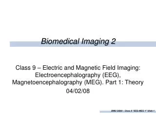
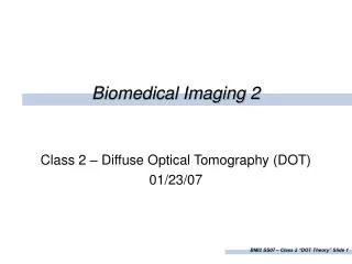
21. (a) (b) (c) Figure 9. Illustration of Morlet wavelet analysis concept. The complex wavelet (solid and dashed sinusoidal curves denote real and imaginary part, respectively) shown in 9(a) is superimposed on the time-varying measurement depicted in 9(b). A new function, equivalent to the covariance between the wavelet and measured signal, as a function of the time point about which the wavelet is centered, is generated. (See Figure 10 for an example of such a computation.) Varying the width of the wavelet, as shown in 9(c), changes the frequency whose time-varying amplitude is computed.

22. Figure 10. Result of wavelet analysis (see Fig. 9) applied to (a) an unmodulated 0.1-Hz sine wave and (b) a frequency-modulated 0.1-Hz sine wave. In 10(a) it is seen that the amplitude and frequency both are constant over time, while in 10(b) it is seen that the amplitude is fixed but the frequency varies.

23. Data “Post-Post-Processing” and “Post-Post-Post-processing”

24. Position Time Starting point: Time Series of Reconstructed Images Physiological parameters: 1) Hboxy, 2) Hbdeoxy, 3) Blood volume 4) HbO2Sat • Temporal Averaging  Spatial Averaging • Spatial Averaging  Temporal Averaging • Wavelet Analysis

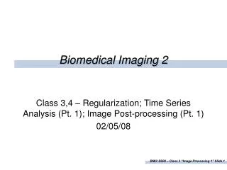
25. (IV) Position temporal integration Spatial map of temporal standard deviation (SD) Baseline temporal mean is 0, by definition (III) Time drop position information spatial integration 100 mean SD Hboxy (II) Hbdeoxy scalar quantities (I) 0 sorted parameter value Method 1: Temporal Spatial Averaging

26. (IV) Position spatial integration Time series of spatial mean → O2 demand / metabolic responsiveness (II) Time Time series of spatial SD → Spatial heterogeneity temporal integration Temporal mean of spatial mean time series: 0, by definition Temporal SD of spatial mean time series Temporal mean of spatial SD time series Temporal SD of spatial SD time series scalar quantities (I) Method 2: Spatial  Temporal Averaging

27. f2 f1 time Method 3: Time-frequency (wavelet) analysis • Starting point is reconstructed image time series (IV) • Use (complex Morlet) wavelet transform as a time-domain bandpass filter operation • Output is an image time series (IV) of amplitude vs. time vs. spatial position, for the frequency band of interest • Filtered time series can be obtained for more than one frequency band • Recompute previously considered Class-II and Class-I results, using Methods 1 and 2, but starting with the wavelet amplitude time series

28. Baseline GTC: Healthy Volunteer Class IV results: normalized wavelet amplitude, right breast Temporal coherence index = 25.7% (26.3% for left breast (not shown))

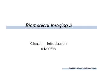
29. Sharp, deep troughs are indicative of strong spatial coordination Baseline GTC: Ductal Carcinoma in Right Breast Class IV results: normalized wavelet amplitude, left (-CA) breast Temporal coherence index = 18.4%

30. Troughs (and peaks) appreciably reduced, or absent Example 2: Ductal Carcinoma in Right Breast Class IV results: normalized wavelet amplitude, right (+CA) breast Temporal coherence index = 13.5%

31. Specificity and Sensitivity Presence of Disease Disease (+) Disease (–) Given disease, what is the probability of a positive test result? True Positive False Positive Test (+) Test Result True Negative False Negative Test (–) Given no disease, what is the probability of a negative test?

32. Predictive Values Presence of Disease Disease (+) Disease (–) Given positive test result, what is the probability of disease? True Positive False Positive Test (+) Test Result True Negative False Negative Test (–) Given negative test result, what is the probability of not having disease?

33. Diagnostic Threshold ROC (Receiver Operating Characteristic) Analysis

34. ROC Curves for Metrics – 1

35. ROC Curves – 2

36. ROC Curves – 3

37. ROC Curves - 4

38. ROC Curves - 5

39. Summary of Calculated Metrics • Data reduction yielded 16 “metrics” • Paired t-tests and ROC curves were used to select metrics that can distinguish between cancer and non-cancer subjects • Selected metrics used in Logistic Regression X:0.01 ≤ p< 0.05, for difference between Cancer and Non-Cancer Subjects XX: p < 0.01

40. Logistic Regression • Binary Distributions (Cancer vs. Non-Cancer) are non-linear • Logistic regression expresses probability of event as a linear combination of “metrics” Xiand coefficientsi

41. New Patient’s Values X1 = .43; X2 = -.05 Logistic Regression Applied Metrics calculated and selected based on t-tests & ROC curves Metrics used as inputs into logistic regression model Probability Logistic regression model calculates i for each metric (Xi) Using i, a predicted probability distribution can be created Metrics Linear Model: P(cancer) = 0.75 New patient’s Xi used to generate probability of cancer in patient Logistic Regression: P(cancer) = 0.90

42. Limitations of Logistic Regression • Metrics Xi must be independent of each other orthogonalization may be needed • Consequently, biologically relevant phenomenology may be ignored by model • Model may be mathematically unstable if the number of cases is low

43. Orthogonalization • The logistic regression model excluded several metrics due to inherent co-linearity (not all are linearly independent) • Transforming excluded metrics to be orthogonal to each other caused a loss of magnitude and of significance • Result using orthogonalized metrics was very similar to original result

44. Final Result • The final predicted probabilities were established by averaging the predicted probabilities for the N=21 and N=37 results • Predicted probabilities for patients within the N = 37 group and not in the N = 21 group were unchanged Combined Metrics (N=21 & N=37)