Download
1 / 54
710 likes | 1.29k Views
OM2. CHAPTER 12. MANAGING INVENTORIES. DAVID A. COLLIER AND JAMES R. EVANS. Chapter 12 Learning Outcomes. l e a r n i n g o u t c o m e s. LO1 Explain the importance of inventory, types of inventories, and key decisions and costs.

E N D
OM2 CHAPTER 12 MANAGING INVENTORIES DAVID A. COLLIER AND JAMES R. EVANS
Chapter 12 Learning Outcomes l e a r n i n g o u t c o m e s LO1Explain the importance of inventory, types of inventories, and key decisions and costs. LO2Describe the major characteristics that impact inventory decisions. LO3Describe how to conduct an ABC inventory analysis. LO4Explain how a fixed order quantity inventory system operates, and how to use the EOQ and safety stock models. LO5Explain how a fixed period inventory system operates. LO6Describe how to apply the single period inventory model.
Chapter 12 Managing Inventories anana Republic is a unit of San Francisco’s Gap, Inc. and accounts for about 13 percent of Gap’s $15.9 billion in sales. As Gap shifted its product line to basics such as cropped pants, jeans, and khakis, Banana Republic had to move away from such staples and toward trends, trying to build a name for itself in fashion circles. But fashion items, which have a much shorter product life cycle and are riskier because their demand is more variable and uncertain, bring up a host of operations management issues. In one recent holiday season, the company had bet that blue would be the top-selling color in stretch merino wool sweaters. They were wrong. Marka Hansen, company president noted, “The No. 1 seller was moss green. We didn’t have enough.” What do you think?Can you cite any experiences in which the lack of appropriate inventory at a retail store has caused you as the customer to be dissatisfied?
Chapter 12 Managing Inventories • Inventoryis any asset held for future use or sale. • The expenses associated with financing and maintaining inventories are a substantial part of the cost of doing business (i.e., cost of goods sold). • Inventory Managementinvolves planning, coordinating, and controlling the acquisition, storage, handling, movement, distribution, and possible sale of raw materials, component parts and subassemblies, supplies and tools, replacement parts, and other assets that are needed to meet customer wants and needs.
Chapter 12 Managing Inventories • Basic Inventory Concepts • Raw materials, component parts, subassemblies, and suppliesare inputs to manufacturing and service-delivery processes. • Work-in-process (WIP) inventoryconsists of partially finished products in various stages of completion that are awaiting further processing. • Finished goods inventoryiscompleted products ready for distribution or sale to customers.
Chapter 12 Basic Inventory Concepts • Basic Inventory Concepts • Cycle inventory (order or lot size inventory) isinventory that results from purchasing or producing in larger lots than are needed for immediate consumption or sale. • Safety stock inventory isan additional amount of inventory that is kept over and above the average amount required to meet demand.
Role of Inventory in the Value Chain Exhibit 12.1
WhereIs Your Inventory? Today, tiny radio frequency identification (RFID) chips embedded in packaging or products allow scanners to track SKUs as they move throughout the store. RFID chips help companies locate items in stockrooms and identify where they should be placed in the store. Inventory on the shelves can easily be tracked to trigger replenishment orders. Recalled or expired products can be identified and pulled from the store before a customer can buy them, and returned items can be identified by original purchase location and date, and whether or not they were stolen. One interesting application has been developed by CVS, a Rhode Island-based pharmacy chain, which is testing RFID technology to inform when a customer has not picked up his or her prescription medicine Chapter 12 Managing Inventories
Chapter 12 Managing Inventories Basic Inventory Decisions • Inventory managers deal with two fundamental decisions: • When to order items from a supplier or when to initiate production runs if the firm makes its own items • How much to order or produce each time a supplier or production order is placed
Chapter 12 Managing Inventories • Inventory Management Decisions and Costs • Four categories of inventory costs: • Ordering or setup costs • Inventory-holding costs • Shortage costs • Unit cost of the stock-keeping units (SKUs)
Chapter 12 Managing Inventories • Inventory Management Decisions & Costs • Ordering costsorsetup costsare incurred as a result of the work involved in placing purchase orders with suppliers or configuring tools, equipment, and machines within a factory to produce an item. • Inventory-holding costsorinventory-carrying costsare the expenses associated with carrying inventory.
Chapter 12 Managing Inventories • Inventory Management Decisions & Costs • Shortage costsorstockout costsarethe costs associated with a SKU being unavailable when needed to meet demand. • Unit costis the price paid for purchased goods or the internal cost of producing them.
Chapter 12 Managing Inventories • Characteristics of Inventory Systems • Number of items: each item is identified by its stock-keeping unit (SKU). • A stock-keeping unit (SKU) is a single item or asset stored at a particular location. • Maintaining data integrity on thousands of SKUs is difficult but must be done. The quality of inventory model decisions is related to the quality of information used in the model(s).
Chapter 12 Managing Inventories • Nature of Demand • Independent demand is demand for an SKU that is unrelated to the demand for other SKUs and needs to be forecast. • Dependant demand is demand directly related to the demand for other SKUs and can be calculated without needing to be forecast. • Deterministic demand is when uncertainty is not included in its characteristics. • Stochastic demand incorporates uncertainty by using probability distributions. • Static demand is stable demand. • Dynamic demand varies over time.
Chapter 12 Managing Inventories • Characteristics of Inventory Systems • Number of time periods in planning horizon: short or long planning horizon such as days, weeks, months, quarters, and years. • Size of time periods: hours, days, weeks, months, quarters. • Thelead timeis the time between placement of an order and its receipt.
Chapter 12 Managing Inventories • Characteristics of Inventory Systems • Astockoutis the inability to satisfy demand for an item. When a stockout happens, the item is either back-ordered or a sale is lost. • Abackorder occurs when a customer is willing to wait for an item. • Alost sale occurs when the customer is unwilling to wait and purchases the item elsewhere.
Chapter 12 ABC Inventory Analysis Inventory Management Infrastructure ABC inventory (Pareto) analysis gives managers useful information to identify the best methods to control each category of inventory (see Exhibits 12.2 to 12.4). A vital few SKUs represent a high percentage of the total dollar inventory value.
Chapter 12 ABC Inventory Analysis • ABC Inventory (Pareto) Analysis • “A” items account for a large dollar value but relatively small percentage of total items (e.g., 10% to 30 % of items, yet 60% to 80% of total dollar usage/value. • “C” items account for a small dollar value but a large percentage of total items (e.g., 50% to 60% of items, yet about 50% of total dollar usage). These can be managed using automated computer systems. • “B” items are between A and C.
Usage-Cost Data for 20 Inventoried Items Exhibit 12.2
ABC Analysis Calculations Exhibit 12.3
ABC Histogram for the Results from Exhibit 12.3 Exhibit 12.4
Chapter 12 Managing Inventories Fixed Quantity System • In a fixed quantity system (FQS),the order quantity or lot size is fixed; the same amount, Q, is ordered every time. • The fixed order (lot) size, Q, can be a box, pallet, container, or truck load. Q might equal 10, 100, or 1,000 units. • Q does not have to be economically determined, as we will do for the EOQ model (described later).
Chapter 12 Managing Inventories Fixed Quantity System • The process of triggering an order is based on the inventory position. • Inventory position (IP)is the on-hand quantity (OH) plus any orders placed but which have not arrived (scheduled receipts, or SR), minus any backorders (BO). • IP = OH + SR – BO [12.1]
Chapter 12 Managing Inventories • Fixed Quantity System • When inventory falls at or below a certain value, r, called the reorder point, a new order is placed. • Reorder point depends on the lead time and nature of demand—oftentimes, the reorder point is selected using the average demand during the lead time (µL). • r = µL = (d) (L) [12.2] • Where d is average demand per unit of time and L is the lead time expressed in the same units of time.
Summary of Fixed Quantity System (FQS) Exhibit 12.5
Fixed Quantity System (FQS) under Stable Demand Exhibit 12.6
Fixed Quantity System (FQS) with Highly Variable Demand Exhibit 12.7
Chapter 12 Managing Inventories Economic Order Quantity Model The Economic Order Quantity (EOQ) model is a classic economic model developed in the early 1900s that minimizes total cost, which is the sum of the inventory-holding cost and the ordering cost. ) ( ( ) average inventory annual inventory holding cost annual holding cost per unit 1 [12.4] = = QCh 2
Economic Order Quantity Model Cost of storing one unit in inventory for the year (denoted by Ch), is given by Ch = (I) (C ), where I is annual inventory-holding charge, C is unit cost of the inventory item, and Q is the number of units in inventory. ) ) ( ) ( ( cost per order number of orders per year annual ordering cost D = [12.5] = Co Q
Cycle Inventory Pattern for the EOQ Model Exhibit 12.8 Average cycle inventory = (maximum inventory + minimum inventory)/2 = Q/2
Chapter 12 Managing Inventories Total Annual Cost: inventory holding cost plus the order (setup cost): 1 D QCh Co TC + = [12.6] Q 2 Optimal Order Quantity: order quantity that minimized the total cost expressed in the equation above. Q* is the quantity that minimizes the total cost and is known as the economic order quantity, or EOQ. √ 2DCo [12.7] Q* = Ch
Chapter 12 Managing Inventories Key Assumptions of EOQ Model • Only a single item (SKU) is considered. • The entire order quantity (Q) arrives in the inventory at one time. No physical limits are placed on the size of the order quantity, such as shipment capacity or storage availability. • Only two types of costs are relevant—order/setup and inventory holding costs.
Chapter 12 Managing Inventories • No stockouts are allowed. • The demand for the item is deterministic and continuous over time. This means that units are withdrawn from inventory at a constant rate proportional to time. For example, an annual demand of 365 units implies a weekly demand of 365/12 and a daily demand of one unit. • Lead time is constant.
Chart of Holding, Ordering, and Total Costs Exhibit 12.9
Safety Stock and Uncertain Demand One way to reduce the risk of a stockout is to add safety stock by increasing the reorder point. A service level is the desired probability of not having a stockout during a lead-time period. For example, a 95 percent service level means that the probability of a stockout during the lead time is .05. Choosing a service level is a management policy decision. Chapter 12 Managing Inventories
When a normal probability distribution provides a good approximation of lead time demand, the general expression for reorder point is r = mL + zsL [12.8] where mL= average demand during the lead time sL= standard deviation of demand during the lead time z = the number of standard deviations necessary to achieve the acceptable service level The term “zsL” represents the amount of safety stock. Chapter 12 Managing Inventories
Chapter 12 Managing Inventories We may not know the mean and standard deviation of demand during the lead time, but only for some other length of time, t, such as a month or year. Suppose that mt and st are the mean and standard deviation of demand for some time interval t, If the distributions of demand for all time intervals are identical to and independent of each other, then mL= mtL [12.9] sL= st √L [12.10]
SolvedProblem Southern Office Supplies, Inc. distributes a wide variety of office supplies and equipment to customers in the Southeast. One SKU is laser printer paper, which is purchased in reams from a firm in Appleton, Wisconsin. Ordering costs are $45.00 per order, one ream of paper costs $3.80, and Southern uses a 20 percent annual inventory-holding cost rate for its inventory. Thus, the inventory-holding cost is Ch = IC = 0.20($3.80) = $0.76 per ream per year. The average annual demand is 15,000 reams, or about 15,000/52 = 288.5 per week, and historical data shows that the standard deviation of weekly demand is about 71. The lead time from the manufacturer is two weeks. Chapter 12 Managing Inventories
Using Equations 12.9 and 12.10, the average demand during the lead time is (288.5)(2) = 577 reams, and the standard deviation of demand during the lead time is approximately 71√2 = 100 reams. The EOQ model results in an order quantity of 1333, reorder point of 577, and total annual cost of $1,012.92. Chapter 12 Managing Inventories
Suppose Southern’s managers desire a service level of 95%, which results in a stockout of roughly once every 2 years. Using the normal distribution tables in Appendix A, we find that a 5 percent upper tail area corresponds to a standard normal z-value of 1.645. That is, the reorder point using Equation (12.8), r, is 1.645 standard deviations above the mean, or r = mL+ zsL= 577 = 1.645(100) = 742 reams This policy increases the reorder point by 742 – 577 = 165 reams, which represents the safety stock. The cost of the additional safety stock is simply Ch times the amount of safety stock, or ($0.76/ream)(165 reams) = $125.40. Chapter 12 Managing Inventories
Chapter 12 Managing Inventories • Fixed Period Systems • An alternative to a fixed order quantity system is a fixed period system (FPS)—sometimes called a periodic review system—in which the inventory position is checked only at fixed intervals of time, T, rather than on a continuous basis. • Two principal decisions in a FPS: • The time interval between reviews (T), and • The replenishment level (M)
Chapter 12 Managing Inventories Fixed Period Systems (no uncertainty) Economic time interval: T = Q*/D[12.8] Optimal replenishment level: M = d (T + L)[12.9] Where d = average demand per time period L = lead time in the same time units M = demand during the lead time plus review period
Summary of Fixed Period Inventory Systems Exhibit 12.10
Operation of a Fixed Period Systems (FPS) Exhibit 12.11
Chapter 12 Special Models for Inventory Management • Fixed Period Systems and the Logic of T + L • In Exhibit 12.11, at the time of the first review, a rather large amount of inventory (IP1) is in stock, so the order quantity (Q1) is relatively small (Q1 = M – IP1). • At the third review cycle, the stock level (IP3) is closer to zero since the demand rate has increased (steeper slope of demand), so the order quantity (Q3 = M – IP3) is much larger and during the lead time, demand was high and some stockouts occurred.
Operation of a Fixed Period Systems (FPS) Exhibit 12.11
Chapter 12 Special Models for Inventory Management • Fixed Period Systems and the Logic of T+L • Note that when an order is placed at time T, it does not arrive until time T + L. Thus, in using a FPS, managers must cover the risk of a stockout over the time period T + L, and therefore, must carry more inventory than in a FQS.
Chapter 12 Special Models for Inventory Management • Single-Period Inventory Model • Applies to inventory situations in which one order is placed for a good in anticipation of a future selling season where demand is uncertain. • At the end of the period, the product has either sold out or there is a surplus of unsold items to sell for a salvage value.
Chapter 12 Special Models for Inventory Management • Single-Period Inventory Model • Sometimes called a newsvendor problem, because newspaper sales are a typical example of the single-period inventory problem. • Problem is solved using technique called marginal economic analysis, which compares loss of ordering one additional item (cs) to the cost of not ordering an additional item (cu) using Equation 12.10. cu cu + cs [12.13] P (demand≤ Q*) =
Solved Problem Let us consider a buyer for a department store who is ordering fashion swimwear about six months before the summer season. The store plans to hold an August clearance sale to sell any surplus goods by July 31. Each piece costs $40 per pair and sells for $60 per pair. At the sale price of $30 per pair, it is expected that any remaining stock can be sold during the August sale. Chapter 12 Managing Inventories