Download
1 / 24
260 likes | 589 Views
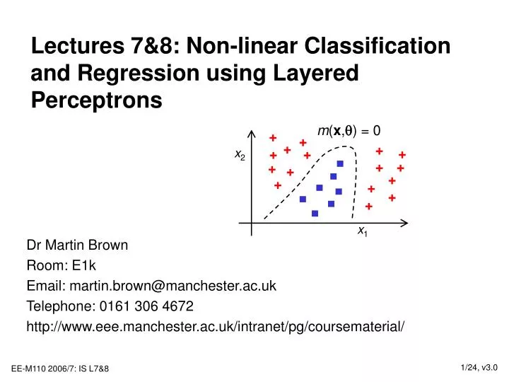
. m ( x , q ) = 0. +. +. . +. +. +. x 2. +. +. . . +. +. +. . +. . +. +. . +. +. +. x 1. Lectures 7&8: Non-linear Classification and Regression using Layered Perceptrons. Dr Martin Brown Room: E1k Email: martin.brown@manchester.ac.uk Telephone: 0161 306 4672

E N D
. m(x,q) = 0 + + . + + + x2 + + . . + + + . + . + + . + + + x1 Lectures 7&8: Non-linear Classification and Regression using Layered Perceptrons Dr Martin Brown Room: E1k Email: martin.brown@manchester.ac.uk Telephone: 0161 306 4672 http://www.eee.manchester.ac.uk/intranet/pg/coursematerial/
Lectures 7&8: Outline • What approaches are possible for non-linear classification and regression problems • Non-linear polynomial networks • Potential and problems using flexible models • Sigmoidal-type non-linear transformations • Modelling capabilities • Regression and classification interpretation • Parameter optimization using gradient descent • Non-linear logical functions and layered Perceptron nets • Lead onto Multi-Layer Perceptron (MLP) models next week
Lecture 7&8: Resources • These slides are largely self-contained, but extra, background material can be found in: • Machine Learning, T Mitchell, McGraw Hill, 1997 • Machine Learning, Neural and Statistical Classification, D Michie, DJ Spiegelhalter and CC Taylor, 1994: http://www.amsta.leeds.ac.uk/~charles/statlog/ • In addition, there are many on-line sources for multi-layer perceptrons (MLPs) and error back propagation (EBP), just search on google • Advanced text: • Information Theory, Inference and Learning Algorithms, D MacKay, Cambridge University Press, 2003
. + + . + + + x2 + + . . + + + . + . + + . + + + x1 Non-Linear Regression and Classification • Most real-world modelling problems are not linear: • A task is non-linear if it cannot be represented using a linear model • Classification the number of classification errors is too large • Regression the noise variance is too large • Using non-linear models/relationships may help to approximate f().
. + + . + + + + + . . . + + + . + . + + . + + + Non-Linear Classification • Consider the following 2-class classification problem • Always compare to prior error rate • Exercise: What are the error rates for prior, optimal linear and non-linear models? • Type of non-linear function is important • Data is generated by (with classification errors): x2 x1
bias model linear model ^ ^ ^ ^ y, y y, y y, y y, y x x non-linear model non-linear interpolation model x x Non-linear Regression • Need to balance model complexity against data accuracy • How much signal is reproducible:
bias linear bilinear quadratic Polynomial Non-Linear Models • A simple and convenient way to extend linear models is to consider polynomial expansions, such as quadratic: • Expansion to any order is possible: cubic, quadratic, subset of terms • Linear model is produced when: • A polynomial model is linear in its parameters • Approximate any continuous function, arbitrarily closely if a high enough polynomial expansion is used (Taylor series)
Example: Quadratic Decision Boundary • A quadratic 2-class classifier is given by: • This has a decision boundary given by: • an 2-dimensional ellipse Example of quadratic classification boundary for the Iris Setosa data Modify Perceptron simulation to work on this?
^ y, y Polynomial Regression “Overfitting” … • Optimal, least squares parameter estimator is given by: • where X is the data matrix, each row represents a data point, each column is one polynomial basis term. • Which polynomial terms should be used - polynomials are flexible but can be quite oscillatory (high frequency components), usually not appropriate Example 20 data points, x randomly drawn from a unit variance, normal distribution, y=exp(-x.^2) , fitted by a fifth order polynomial.
Sigmoidal Non-Linear Transformations • Lets consider another way to introduce non-linearities into a basic linear model, by producing a continuous, non-linear transformation of a weighted sum: • What sort of single input, single output functions, f(), are possible? • To estimate parameters using gradient descent, it should be differentiable • To use for classification and regression, is should be able to represent linear and step functions, as appropriate x0=1 q0 y x1 q1 qn xn
f(u) u Tanh() Function • Consider the tanh() function whose output lies in (-1,1) • When there is a single input: u = q0+xq1 • When q1 is large (= 4) • Almost a step function • When q1 is small (= 0.25) • Almost a linear relationship • q0 shifts tanh() horizontally q1 large q1 small
Tanh Function in 2D X-Space • Such functions are often known as ridge functions, because they are constant along a line in input space! • u = xTq = c
0-1 Sigmoid • Many books/notes use the following sigmoid function: • which has an output lying in the range (0,1). • In these notes, we’ll refer to both transformation functions as sigmoidal functions, because of their “lazy S” shape • In fact, they’re just transformations of each other:
Sigmoidal Parameter Estimation • Gradient descent update for a single training datum: • For the ith training pattern: • Using the chain rule: • Giving an update rule: Similar to the LMS rule, apart from the extra sigmoidal derivative term, f’().
df/du f(u) Sigmoidal Parameter Estimation (ii) • Sigmoidal function’s derivative (tanh):
Layered Perceptron Networks • In this section, we’re going to consider how these sigmoidal nodes can be connected together into layers to give greater/more flexible non-linear modelling behaviour • Two central questions: • What are the non-linear modelling capabilities? • How to estimate the non-linear parameters? x0 h0 y h1 x1 x2 h2
1 -1 0 1 1 0 x Linearly Separable 2D Logical Functions • Note class output values of 0 and 1 in next few slides • AND • OR • NOT 1 1 1 -1 -1 1 x2 x2 -1 0 -1 -1 -1 0 1 x1 1 0 0 x1 1 1 1 1 1 1 x2 x2 1 0 -1 1 -1 0 1 x1 1 0 0 x1 -1 1 x
-1 1 1 -1 1 1 x2 x2 1 0 -1 1 -1 0 1 x1 1 0 0 x1 Nonlinearly Separable 2D XOR • eXclusive OR (XOR) - n bit parity: • 2 inputs: • Data generated by: • y = (NOT x2 AND x1) OR (NOT x1 AND x2). • Non-linear, polynomial input transformations: • x3 = x1*x2, makes the problem separable • How can multi-layer networks?
Multi-Layer Network for 2D XOR • Can be implemented as a two layer network (two layers of adjustable parameters) with two “hidden nodes” in the hidden layer • Empty circles represent linear Perceptron nodes • Solid circles represent a real signals • Arrows represent model parameters q • (NOT x2 AND x1) OR (NOT x1 AND x2) • Is represented in a 2 layer network as: • h1: (NOT x2 AND x1) • h2: (NOT x1 AND x2), y = h1 OR h2 x0=1 h0=1 y h1 x1 x2 output layer h2 hidden layer
x0=1 h0=1 y h1 x1 x2 output layer h2 hidden layer Exercise: Determine the 9 Parameters • Write down the parameter vectors for the 3 Perceptron nodes • h1: (NOT x2 AND x1) • h2: (NOT x1 AND x2), • y: h1 OR h2
Logical Functions and DNF • Any logical function can be expressed as the union of “negation and conjunction” terms. • It can be realized with a 2 layer Perceptron network. • Each hidden layer unit to respond to exactly one positive example. • Output layer is formed from the union of the hidden layer outputs. • f = h1 OR h2 OR … OR hP • Each data point/positive example is given its own “hidden unit”, which responds to only that point • Essentially, it memorizes the positive training samples
Lecture 7&8: Conclusions • There are many ways to build and use non-linear models for classification and regression purposes • Potentially get more accurate predictions/fewer errors if the data is generated by a non-linear relationship • Parameter estimation is sometimes more complex • No direct optimal parameter calculation • Gradient-based estimation has local minima and differing curvatures • Need to select an appropriate non-linear framework Multi-layer (sigmoidal) Perceptrons are one such framework • Non-linearity controlled by nodes in hidden layer • Parameters estimated using gradient descent • Several factors need to be considered
Lecture 7&8: Laboratory (i) • Matlab • Extend the basic Perceptron matlab script so that it now trains up a quadratic classifier (note that the plotting routines will no longer be appropriate). • Implement the sigmoidal perceptron learning algorithm, where the model consists of a single layer with a tanh activation function and the parameters are updated after each presentation of a datum (see Slides 10-14) • Test the algorithm on the logical AND and logical OR data, as you did for the normal Perceptron algorithm in the laboratory in IS2.ppt • What are the similarities/differences of this model compared to the normal Perceptron algorithm described in IS2.ppt
Lecture 7&8: Laboratory (ii) • Theory • Prove the relationship on Slide 13 between the two types of sigmoids • Verify the derivative of the tanh function on Slide 15, and prove that the derivative of the (0,1) sigmoid on Slide 13 can be expressed as y(1-y) • Calculate the optimal parameter values missing on Slides 17 and 20. • Derive a generic rule for setting the parameter values on Slide 21 for an arbitrary logical function. You may assume that you know the number of positive examples, the number of features and the logical structure of each positive example