Download
1 / 37
370 likes | 450 Views
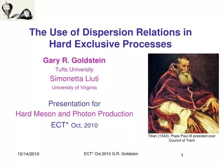
The Use of Dispersion Relations in Hard Exclusive Processes. Gary R. Goldstein Tufts University Simonetta Liuti University of Virginia Presentation for Hard Meson and Photon Production ECT* Oct, 2010. Titian (1543)- Pope Paul III presided over Council of Trent. 10/14/2010.

E N D
The Use of Dispersion Relations in Hard Exclusive Processes Gary R. Goldstein Tufts University Simonetta Liuti University of Virginia Presentation for Hard Meson and Photon Production ECT*Oct, 2010 Titian (1543)- Pope Paul III presided over Council of Trent 10/14/2010 ECT* Oct.2010 G.R. Goldstein 1
Outline of Discussion Dispersion Relations, DVCS & GPDs - DGLAP & ERBL • Thresholds & DRs • Unitarity & analyticity • Threshold limits • Kinematic restrictions • Model calculations • ERBL region & partons • Intermediate states • “semi-disconnected” diagrams • Non-replacement for >0 See: GG, Liuti, PRD80, 071501 (2009). GG, Liuti, ArXiv hep-ph/1006.0213 10/14/2010 ECT* Oct.2010 GR.Goldstein 2
Are GPDsHeretical? Pasquale Cati (1588)- Council of Trent with Church Triumphant
Phenomenological Constraints on GPDsGPD challenge - How unique?Models; Parameterizations; Theoretical constraints Constraints from PDFs Form factors: • Further Constraints: • Polynomiality Sensible hadron shape at x~1 • & x→0 Regge behavior Sensible prediction for t dependence - positivity • see Ahmad, Liuti et al. (AHLT) (2008,09) • & ongoing work (S.Liuti, GG, O. Gonzalez Hernandez in this session) • (Connection with TMDs? Wigner distributions? Beyond models?) ECT* Oct.2010 GR.Goldstein 4
What about Analyticity? GPDs are real functions of x,,t,Q2. Functions of many variables - complex x not & t? Connection of Dispersion Relations to GPDs? Consider Virtual Compton scattering from hadronic view. q γ * q′ γ q(Q2) q′ γ * γ γ ∫dk -d2kT XP+,kT (X-ζ)P+,kT -ΔT N GPD P+ N′ N N′ N t (1-ζ)P+,-ΔT Factorized “handbag” parton picture Convert kinematics s-channel unitarity hadron picture Imaginary part for on-shell intermediate states 10/14/2010 ECT* Oct.2010 GR.Goldstein 5
Dispersion relations: constraints on GPD modeling & experimental extraction • Deeply Virtual Compton Scattering (DVCS) amplitudes satisfy unitarity, Lorentz convariance & analyticity (Long history - 1950’s, forward, fixed t, Lehmann ellipse, double DRs & Mandelstam Rep’n, Regge poles, duality, . . . ) • (Generic) T(ν,t,Q2) (ν=(s-u)/4M) has ν or s & u analytic structure determined by nucleon pole & hadronic intermediate on-shell states - completeness dσ/dt ∝ |T(ν,t,Q2)|2 s-channel unitarity hadron picture Imaginary part for on-shell intermediate states 10/14/2010 ECT* Oct.2010 GR.Goldstein 6
Hadron to parton variables: s=(P+q)2=M2-Q2+2MνLab ν=(s-u)/4M=(2s+t+Q2-2M2)/4M = νLab+(t - Q2)/4M xBJ= Q2/2MνLab , X=k⋅P/q⋅P, ζ=q⋅P′/q⋅P ξ=ζ/(2-ζ), x=(2X-ζ)/(2-ζ) ξ=Q2/4Mν Integration variable x=Q2/4Mν′ • Teryaev; Anikin & Teryaev; Ivanov & Diehl; Vanderhaeghen, et al.; Müller, et al.; Brodsky, et al. Compton Form Factor 10/14/2010 ECT* Oct.2010 GR.Goldstein 7
Dispersion Relations (Anikin, Teryaev, Diehl, Ivanov, Vanderhaeghen…) G.Goldstein and S.L.,PRD’09 H(x,x,t) + C(t) All information contained In the “ridge” x=? Branch cut -1<x<+1. (graph: D. Müller) ECT* Oct.2010 GR.Goldstein
Dispersion Theory The amplitudes are analytic --in the chosen kinematical variables, , xBj, ,s -- except where the intermediate states are on shell k’+=(X-)P+ k+=XP+ P+ PX+=(1-X)P+ DIS cut epeX pole, =Q2/2M epe’p ECT* Oct.2010 GR.Goldstein
OPE is seeded in DRs (see e.g. Jaffe’s SPIN Lectures) From DR + Optical Theorem =1/x to Mellin moments expansion ECT* Oct.2010 GR.Goldstein
DVCS: Where is the threshold?G.Goldstein and S.L., PRD’09 Because t 0, the quark + spectator’s kinematical “physical threshold” does not match the one required for the dispersion relations to be valid Continuum threshold • Continuum starts ats =(M+m)2 lowest hadronic threshold. ECT* Oct.2010 GR.Goldstein
Where is threshold? • Imaginary part from discontinuity across unitarity branch cut - from ν threshold for production of on-shell states - e.g. πN, ππN, ππΔ, etc. • Continuum starts at s =(M+mπ)2 ⇒ lowest hadronic threshold. • Physical region for non-zeroQ2 and t differs from this. • How to fill the gap? ν0 νphysical ν t s=(M+mπ)2 10/14/2010 ECT* Oct.2010 GR.Goldstein 12
ν Q2=1.0 GeV2 νPhysical -t s=(M+mπ)2 B.Pasquini, et al.,Eur.Phys.J.A11,185 (2001) 10/14/2010 ECT* Oct.2010 GR.Goldstein 13
Gaps in dispersion integrals ν ν Q2=2.0 GeV2 Q2=1.0 GeV2 -1.1>t>-2.7 GeV2 Physical region has no gap for Q2=2.0 GeV2 νPhysical νPhysical s=(M+mπ)2 -t -t s=(M+mπ)2 -0.60>t>-1.34 GeV2 Physical region has no gap for Q2=1.0 GeV2 ν Q2=5.5 GeV2 -2.4>t>-7.4 GeV2 Physical region has no gap for Q2=5.5 GeV2 νPhysical M+2mπ next threshold . . . M+nmπ, etc. s=(M+mπ)2 -t 10/14/2010 ECT* Oct.2010 GR.Goldstein 14
Physical threshold obtained by imposing T2 > 0 (same as tmin = -M2 2/(1-)2) ν physical Q2=2.0 GeV2 νPhysical s=(M+mπ)2 -t continuum • How does one fill the gap? Analytic continuation?…problem for experimental extraction. • Range of x limited experimentally. • What is reasonable scheme for continuation? Model dependence. ECT* Oct.2010 GR.Goldstein
10/14/2010 ECT* Oct.2010 GR.Goldstein 16
Crossing symmetry Analyticity in the energy variable ν=(s-u)/4M ∝ 1/x requires crossing (anti)symmetric amplitudes. At GPD level need: H (+) (x,ξ,t ) = H (x,ξ,t) − H (−x,ξ,t) H (−) (x, ξ ) = H (x,ξ,t) + H (−x,ξ,t) singlet non-singlet Each is multiplied by hard part from γ* q→γ q’ C ±(x/ξ) = 1 /(−X + ζ − iϵ) ∓ 1/ (X − iϵ) or 1/(ξ – x − iϵ) ∓ 1/(ξ + x − iϵ) H(+)(ν,t)∝ναP(t)-1whereαPomeron(0)=1+δ H(-)(ν,t)∝ναR(t)-1where αRegge(0)≈1/2 DR needs subtraction Unsubtracted DR ECT* Oct.2010 GR.Goldstein 17
Examples of DVCS dispersion integrals & threshold dependences Regge form for H(X,ζ,t) or HR(ν,Q2,t) = β(t,Q2)(1-e-iπα(t))(ν/ν0)α(t) So ReHR(ν,Q2,t) = tan(πα(t)/2) ImH(ν,Q2,t) Dispersion: This is exact for νThreshold=0. For Q2 , νThreshold = -t/4M this is asymptotic. 10/14/2010 ECT* Oct.2010 GR.Goldstein 18
10/14/2010 ECT* Oct.2010 GR.Goldstein 19
Diquark spectator model - simple, no spin Valence quark model Based on Brodsky & Llanes-Estrada model q′ q γ * γ ζ=0.12 t = -0.5,-1.0,-2.0 GeV2 k k′ X ERBL region DGLAP region P′ P N′ N No symmetry around x=0 or X=ς/2 scalar diquark - subprocess û-channel pole with nucleon→quark+diquark form factors 10/14/2010 ECT* Oct.2010 GR.Goldstein 20
Scalar diquark, polynomiality & DR H(x,x,t=-0.5 GeV2) x2 moment of H(x,ξ,t) vs. ξfor 3 t values ξ 10/14/2010 ECT* Oct.2010 GR.Goldstein 21
10/14/2010 ECT* Oct.2010 GR.Goldstein 22
Dispersion relations for AHLT GPDs Real part H(ζ,t) for Q2=5.5 GeV2 Evolved H(X,ζ,t) from low Q2 scale, then get Im H (ζ,t) or H(X,X,t) & direct integration for Re H (ζ,t) 10/14/2010 ECT* Oct.2010 GR.Goldstein 23
Dispersion relations cannot be directly applied to DVCS because one misses a fundamental hypothesis: “all intermediate states need to be summed over” • For DVCS one is forced to look into the nature of intermediate states because there is no optical theorem • This happens because “t” is not zero and there is a mismatch between the photons initial and final Q2 t-dependent threshold cuts out physical states “counter-intuitively as Q2 increases the DRs start failing because the physical threshold is farther away from the continuum” ECT* Oct.2010 GR.Goldstein
Dispersion Direct Regge Model Difference Direct Dispersion ECT* Oct.2010 GR.Goldstein
When deeply virtual processes involve directly final states - as in exclusive or semi-inclusive processes - “standard kinematic approximations should be questioned” (Collins, Rogers, Stasto, 2007, Accardi, Qiu, 2008) H is calculated off the ridge ECT* Oct.2010 GR.Goldstein
Summary of part 1: dispersion relations cannot be applied straighforwardly to DVCS Need model for continuation into unphysical regions.. The “ridge” does not seem to contain all the information. ECT* Oct.2010 GR.Goldstein
DVCS Kinematics q q'=q+ k+=XP+, kT k'+=(X- )P+, kT- T P'+=(1- )P+, - T P+ What about X= -- returning quark with no + momentum (stopped on light cone) & X< “central” or ERBL region How to interpret? ERBL similar to contributions other than the parton model mentioned by Jaffe (1983) ECT* Oct.2010 GR.Goldstein
Interpreting off-forward GPDs see Jaffe NPB229, 205(1983) For pdf’s - forward elastic Relate T-product to cut diagrams partons emerge + Completeness ECT* Oct.2010 GR.Goldstein
Singularities in covariant picture along with s and u cuts X> Im k- X< Im k- 1' 3' 1' 2' 3' 2' Re k- Re k- Diquark spectator on-shell struck quark on-shell Returning quark =outgoing anti-q 2 3 1 ECT* Oct.2010 GR.Goldstein
In DGLAP region spectator with diquark q. numbers is on-shell k’+=(X-)P+ k+=XP+ P’+=(1- )P+ P+ PX+=(1-X)P+ In ERBL region struck quark, k, is on-shell k’+=(-X)P+ P’+=(1- )P+ P+ Analysis done for DIS/forward case by Jaffe NPB(1983) In forward kinematics can use alternative set of connected diagrams that have partonic interpretation. ECT* Oct.2010 GR.Goldstein
ERBL region corresponds to semi-disconnected diagrams: no partonic interpretation What is meaning of diagram? note: Diehl & Gousset (‘98) - for off-forward generalization of Jaffe’s argument, still can replace T-ordered †(z) (0) with cut diagrams & interpret ERBL region as q+anti-q k’+=(-X)P+ P’+=(1- )P+ P+ ECT* Oct.2010 GR.Goldstein
Is there a way to restore a partonic interpretation? We consider multiparton configurations FSI A B 2' 3 3' 2 l+=(X-X')P+ = y P+ k'+=(X'- )P+ k+=XP+ 1 1' P'+=(1- )P+ P+ PX+=(1-X)P+ P'X+=(1-X')P+ Planar k+=XP+ P+ PX+=(1-X)P+ ECT* Oct.2010 GR.Goldstein
A A B B 2' 3 2' 3 3' 3' 2 2 k'+=(X'- )P+ k'+=(X'- )P+ l+=(X-X')P+ = y P+ l+=(X-X')P+ = y P+ k+=XP+ k+=XP+ 1 1 1' 1' P'+=(1- )P+ P'+=(1- )P+ P+ P+ PX+=(1-X)P+ PX+=(1-X)P+ P'X+=(1-X')P+ P'X+=(1-X')P+ Non-Planar FSI“promotion” k+=XP+ k+=XP+ P+ P+ PX+=(1-X)P+ PX+=(1-X)P+ ECT* Oct.2010 GR.Goldstein
Summary of part 2: GPDs in ERBL region can be described within QCD, consistently with factorization theorems, only by multiparton configurations, possibly higher twist. ECT* Oct.2010 GR.Goldstein
Lessons from examples • Moderate reach of Eγ (Jlab<12 GeV) or s<25 GeV2=(5 GeV)2 not far from t-dependent thresholds • Non-forward dispersion relations require some model-dependent analytic continuation • Difference between direct & dispersion Real H(ζ,t) depends on thresholds • DVCS & Bethe-Heitler interference via cross sections & asymmetries measures complex H(ζ,t) directly Interpreting ERBL • “partonic” picture unclear - higher twist? FSI? • N q+anti-q +N’ ? • N Meson + N’ ? • ERBL region exists. Significance? Model using (anti)symmetric form &/or fsi. 10/14/2010 ECT* Oct.2010 GR.Goldstein 37