Download
1 / 18
200 likes | 503 Views
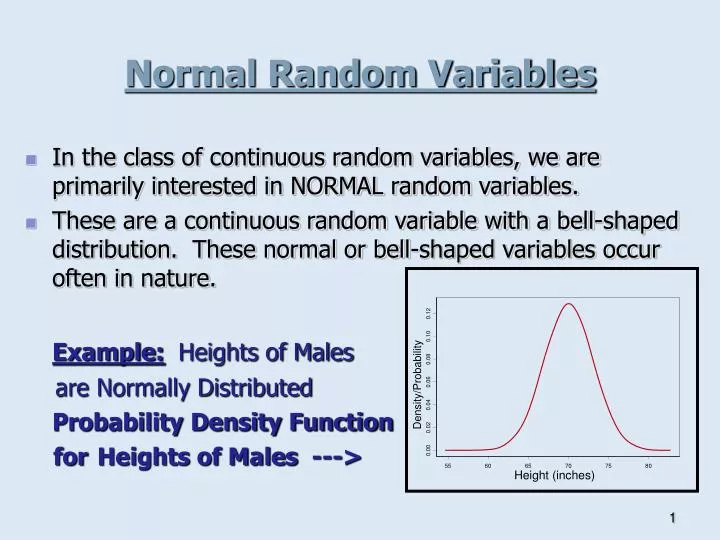
Normal Random Variables. In the class of continuous random variables, we are primarily interested in NORMAL random variables. These are a continuous random variable with a bell-shaped distribution. These normal or bell-shaped variables occur often in nature. Example: Heights of Males

E N D
Normal Random Variables • In the class of continuous random variables, we are primarily interested in NORMAL random variables. • These are a continuous random variable with a bell-shaped distribution. These normal or bell-shaped variables occur often in nature. Example:Heights of Males are Normally Distributed Probability Density Function for Heights of Males --->
Properties of the Normal distribution • There are infinitely many normal pdf’s (curves). To fully describe a normal curve, we need the location (mean, μ) and the spread (standard deviation, σ). • Notation: If X a normal random variable with mean E(X)=μ and variance Var(X)=σ2we write X~N (μ, σ2) For population mean and s.d. we use the Greek letters μ and σ, for the sample mean and s.d. we use and s. • The distribution is symmetrical around the mean μ. • The median, and the mean are equal due to the symmetry of the distribution. • The total area under the curve is equal to one.
The parameters µ and σ For all, σ=1 For all, µ =0 σ=1/2 µ=0 µ=2 µ=-2 σ=1 σ=2
Probabilities with Normal RVs • When we consider Normal Random Variables (or any continuous r.v.), we are interested in the probability that Xfalls into some INTERVAL. • The probability a random variable X~N(μ, σ2) to take a value is equal to zero. In other words, if X~N(μ, σ2) then P(X=k)=0, where k is some number. Example:Suppose X is the height of a randomly chosen college woman. Further suppose that the heights of college women can be described as a normal, with μ = 65inches (in), and σ = 2.7 in. We might ask: • What is the proportion of women that are shorter than 62 in? • What is the probability that X is between 65 and 67in?
Graphical Representation of Probabilities P(65<X<67) P(X<62) • The total area under the curve is equal to 1! • The probability that X falls in an interval is equal to the area of the region below the curve and over the interval.
Probabilities with Normal RVs • The total area under the curve is equal to 1! • The probability that X falls in an interval is equal to the area of the region below the curve and over the interval. • For example P(a X b) is equal to the area under the curve between a and b. • Due to the continuity of the normal distribution we have that the probability a normal random variable to take a value is equal to zero, thus P(X a)= P(X < a) P(a X b)= P(a < X < b) P(a X < b)= P(a < X < b) etc.
Standard Normal Distribution • A normal r.v. with µ=0 and σ=1 is called a standard normal random variable. • We denote it with Z, so that Z~N(0,1). • We have tables for the probabilities of the form P(Z < z) where z ≥0. e.g. P(Z ≤ 0.5), P(Z < 2). • Probabilities of the form P(Z < - 0.4), P(Z > 1.2), P(Z > - 0.25) have to be transformed into probabilities of the form P(Z < z) where z ≥ 0.
How to use the table • The probability P(Z<1.14) is the number in the table where the row of 1.1 and the column of .04 are crossed. Thus, P(Z<1.14)=0.8729 • More examples: P(Z<0.57)=.7157 P(Z<2)=.9972 P(Z<1.3)=.9032 P(Z<0)=0.5
Calculating Probabilities of Z~N(0,1) For Z~N(0,1), and α≥0: • P(Z > α) =1-P(Z < α) • P(Z < -α) =1-P(Z < α) • P(Z > -α) =P(Z < α) • P(b <Z < c) =P(Z < c) - P(Z < b), for any b and c. Draw a normal curve and shade the areas corresponding to the above probabilities.
Calculating Probabilities of any normal r.v. X~N( µ , σ) We can obtain any type of probabilities of interest for any normal r.v X~N(μ, σ 2) by first transforming X into Z using the following “standardization theorem’:
How to Calculate Probabilities If you want P(X < x), first compute the z-score: z = (Value – mean)/(Standard Deviation) = (x-µ)/σ, But P(X < x) = P(Z < z) for which we have tables!! Example: X = height of a college woman, X~N( 65, 2.72) 1.P(X < 62) z = (62 – 65)/2.7 = -3/2.7 = -1.11 P(X < 62) = P(Z < -1.11) (now use Normal Table) = 0.134 = 13.4% 2.P(65 < X < 67) z1 = (65 – 65)/2.7 = 0, z2 = (67 – 65)/2.7 = 1.11 P(65 < X < 67) = P(0 < Z < 1.11) = P(Z < 1.11) – P(Z < 0) = .867 – .5 = .367 or 36.7% 3.P(X>62) = 1-P(X<62) = 1-0.134 = 0.866
Example: Suppose verbal SAT scores of high-school freshman are normally distributed with a mean of 500 and a standard deviation of 50. • What is the probability of a randomly chosen individual having a score greater than 600? z-score = [600-500]/50 = 2 P(X>600) = P(Z>2) = 1- P(Z 2)= 1-P(Z<2) = 1-.9772 = 0.228 Note that the only difference in the two graphs below is the scale on the tow axes. However, the shaded areas are equal…since the total area under any of this curves is one. P(X>600) P(Z>2) -4 -2 0 2 4
What is the probability of a randomly chosen individual having a score between 400 and 500? We want P(400<X<500). z-score1 = z1 = [400-500]/50 = -2 z-score2 = z2 = [500-500]/50 = 0 P(400<X<500) = P(-2 < Z < 0) = P(Z<0) – P(Z<-2) = .5-.228 = .4772 (from Table) P(-2<Z<0) That is the probability of a randomly chosen student having a score between 400 and 500 is about .48 or 48%.
What is the probability of a randomly chosen individual having a score between 350 and 450? z-score1 = z1 = [350-500]/50 = -3 z-score2 = z2 = [450-500]/50 = -1 P(350<X<450) = P(-3 < Z < -1) = P(Z<-1) – P(Z<-3) = .1587-.0013 = .1574 (from normal Table) P(-3<Z<-1) That is the probability of a randomly chosen student having a score between 350 and 450 is about .16 or 16%.
The Empirical Rule states that for any bell-shaped distribution, approximately 68% of the values fall within 1 standard deviation of the mean in either direction. (in the interval μ ± σ) 95% of the values fall within 2 standard deviations of the mean in either direction. (in the interval μ ± 2σ) 99.7% of the values fall within 3 standard deviations of the mean in either direction. (in the interval μ ± 3σ) This empirical rule is valid for all bell-shaped distributions but it is exactly right in the case of the normal distribution. Check the following probabilities: P(-1<Z<1) = ___ , P(-2<Z<2) =___ , P(-3<Z<3) =___ The Empirical Rule and Normal Distrib.
How can we find percentiles? • Question: For a normal r.v. X with mean μ and standard deviation σ , how can we find x (a value of X ), such that P( X ≤ x) = α%, where α is α known probability. e.g. if α = 95 , the 95th percentile of X is the value of X such that 95% of its possible values are less than that. • Solution: First we get the α-th percentile for Z, P(Z≤ z) = 0.95 gives z = 1.64. and we get x using x= σ z + μ. • Example: What is the 90th percentile of the height of college women? [Recall that X~N( 65, 2.72)] • P(Z≤ z) = 0.90, then z = 1.38 since P(Z<1.38)=0.8997 the closest value to 0.90 in the table. • x=2.7*1.38+65=68.726, • Thus the 90th percentile of the height of college women is 68.726in.
SummaryDefinitions and theory for Normal r.v’s. • Knowing μ and σ, specifies the particular normal distribution out of the class of all normal distributions. • The pdf of any normal r.v X~N(μ , σ2), also called normal curve, is symmetric, bell shaped and centered at μ. • The standard normal random variable, Z, has μ = 0 and σ2 = σ =1. • We have the tables for all the probabilities of the form P(Z ≤ z) = P(Z < z). • For any normal r.v X ~ N(μ , σ2 ), we can obtain any probabilities of interest using the “standardization theorem’: P(X ≤ x) = P [(X- μ)/ σ ≤ (x- μ)/ σ] = = P(Z ≤ z), Where z = (x- μ)/ σ, is called the z-score of x.
SummaryFinding Probabilities of X~N(μ , σ2 ) • First find the z-score of x (or x’s if more than one) to be able to use the tables. • Write the probability in terms of Z. • Think what is the area under the curve that corresponds to this probability • Having in mind that the normal curve is symmetric and that the total area under the curve is equal to 1 figure out how to transform this probability into the form P(Z<z) [rules on slide ]. • Finally, obtain the probability using the table. • To find the α-th percentile of X : • We want to find x (a value of X), such that P( X ≤ x) = α% • First we get the α-th percentile for Z, =for example ifα=95) • P(Z≤ z) = 0.95, then z = 1.64 • We get x using x= σ z + μ