Download
1 / 65
650 likes | 770 Views
Paul Fischer Mathematics and Computer Science Division Argonne National Laboratory. Hisham Bassiouny, Henry Tufo University of Chicago Francis Loth, Seung Lee University of Illinois, Chicago Jerry Kruse Juniata College

E N D
Paul Fischer Mathematics and Computer Science Division Argonne National Laboratory Hisham Bassiouny, Henry Tufo University of Chicago Francis Loth, Seung Lee University of Illinois, Chicago Jerry Kruse Juniata College Julie Mullen Worcester Polytechnic Inst. fischer@mcs.anl.gov www.mcs.anl.gov/~fischer
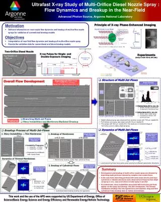
Accurate simulation of long-time dynamics pattern formation in nonequilibrium flows convection dynamics in deep atmospheres transitional boundary layers heat transfer enhancement vascular flows Motivation: Spectral Element Simulations
Outline • Temporal/Spatial Discretization • Spectral element method • Filter-based stabilization • Computational complexity - pressure solve • Pressure projection • Overlapping Schwarz • Transition in vascular flows
Navier-Stokes Equations • Reynolds number Re ~ 1000 - 2000 • small amount of diffusion • highly nonlinear (small scale structures result) • Time advancement: • Nonlinear term: explicit (3rd-order AB or characteristics) • Stokes problem: pressure/viscous decoupling: • 3 Helmholtz solves for velocity • (consistent) Poisson equation for pressure • Filter velocity field at end of each time step for stability (FM 2001)
Characteristics-Based Convection Treatment(OIFS Scheme - Maday, Patera, Ronquist 90, Characteristics - Pironneau 82)
Unsteady Stokes Problem at Each Step • linear (allows superposition) • implicit (large CFL, typ. 2-5) • symmetric positive definite operators (conjugate gradient iteration)
Spatial Discretization: Spectral Element Method (Patera 84, Maday & Patera 89) • Variational method, GL quadrature. • Domain partitioned into K high-order quadrilateral (or hexahedral) elements (decomposition may be nonconforming - localized refinement) • Trial and test functions represented as Nth-order tensor-product polynomials within each element. (N ~ 4 -- 15, typ.) • KN 3gridpoints in 3D, KN 2gridpoints in 2D. • Converges exponentially fastwith N for smooth problems. 3D nonconforming mesh for arterio-venous graft simulations: K = 6168 elements, N = 7
N = 4 N = 10 Examples of Local Spectral Element Basis Functions in 2D Nth-order Lagrangian interpolants based on the Gauss-Lobatto-Legendre quadrature points in [-1,1]2
PN - PN-2 Spectral Element Method for Navier-Stokes (MP 89) Velocity, uin PN , continuous Pressure,p in PN-2 , discontinuous Gauss-Lobatto Legendre points (velocity) Gauss Legendre points (pressure)
Spectral Convergence - Analytic Navier-Stokes Solution (Kovasznay, 1948)
Numerical dispersion as a function of polynomial degree Convection of non-smooth data on a 32x32 grid (K1 x K1 spectral elements of order N). (cf. Gottlieb & Orszag 77)
Stabilization essential for high Reynolds number flows At end of each time step, Interpolate u onto GLL points for PN-1 Interpolate back to GLL points for PN Results are smoother with linear combination: (F. & Mullen 01) Preserves interelement continuity and spectral accuracy Equivalent to multiplying by (1-a)the Nth coefficient in the expansion u(x) = Sukvk(x)(Boyd 98) vk(x):= Lk(x) - Lk-2(x) Filter-Based Stabilization (Gottlieb et al., Don et al., Vandeven, Boyd, ...) F1(u) = IN-1 u Fa (u) = (1-a)u + aIN-1 u (a ~ 0.05 - 0.2)
Numerical Stability Test: Shear Layer Roll-Up (Bell et al. JCP 89, Brown & Minion, JCP 95, F. & Mullen, CRAS 2001) 2562 2562 1282 2562 2562 1282
Error in Predicted Growth Rate for Orr-Sommerfeld Problem at Re=7500 Spatial and Temporal Convergence (FM, 2001) Base velocity profile and perturbation streamlines
1D Steady-State Convection-Diffusion Equation • ux = m uxx + f , x c [0,1], f =1 • Galerkin formulation is unstable when the number of degrees-of-freedom is odd and m t0 [Canuto 88]. • For steady convection-diffusion equation: N=16 N=15 Solid - unfiltered Dashed - filtered
Filter-Based Stabilization • For unsteady convection-diffusion equation: • ut + ux = m uxx + f , x c [0,1], f =1 • can show that steady state discrete solution for • the filtered problem satisfies • (m A + C + H (Fa-1- I))u = B f • where • A = SEM Laplacian • C = (skew symmetric) convection operator • H = discrete Helmholtz operator (m A + B/Dt) • B = SEM mass matrix • The term H (Fa-1- I)controls the singular mode when m t0 • and the number of degrees of freedom is odd (N even).
Filter-Based Stabilization • Note that filtering only the (nonlinear) convective term is insufficient to provide stability. • For example, for the unsteady convection-diffusion equation one has: • Hun+1 = (Dt -1 B - Fa C )un +B f • which solves the steady state problem • (m A + Fa C)u = B f • In this case, there is no stability when m t0 since Fa C is singular when the number of degrees of freedom is odd (N even).
Re = 700 blow up Filtering permits Red99 > 700 for transitional boundary layer calculations Re = 1000 Re = 3500
Consistent Splitting for Unsteady Stokes(MPR 90, Perot 93, Couzy 95) • E- consistent Poisson operator for pressure, SPD • boundary conditions applied in velocity space • preconditioned with overlapping Schwarz method (Dryja & Widlund 87, PF 97, FMT 00)
Computational Complexity • Pressure solve, Epn = gn, most expensive step. • Remedies: • Compute best fit, p*, in space of previous solutions: • || pn -p*||E[ || pn -q||E for all q in span{pn-1, . . . , pn-l} • two additional matrix-vector products per step (very cheap) • Solve for perturbation, pn -p*, using overlapping Schwarz PCG • tensor-product based local solves • fast parallel coarse-grid solve using sparse-basis projection
Initial guess for Axn = bn via projection • || xn -x*||A= O(Dtl) + O( etol ) • two additional mat-vecs per step • storage: 2+lmax vectors • results with/without projection (1.6 million pressure nodes)
Overlapping Schwarz Precondtioning for Pressure (Dryja & Widlund 87, Pahl 93, PF 97, FMT 00) K S k =1 z = P-1r = R0TA0-1 R0 r+ Ro,kTAo,k-1 Ro,k r Ao,k - low-order FEM Laplacian stiffness matrix on overlapping domain for each spectral element k (Orszag, Deville & Mund, Casarin) Ro,k - Boolean restriction matrix enumerating nodes within overlapping domain k A0 - FEM Laplacian stiffness matrix on coarse mesh (~ K x K ) R0T - Interpolation matrix from coarse to fine mesh
d Overlapping Solves: Poisson problems with homogeneous Dirichlet bcs. Coarse Grid Solve: Poisson problem using linear finite elements on spectral element mesh (GLOBAL). Two-Level Overlapping Additive Schwarz Preconditioner
Overlapping Schwarz - local solve complexity • Exploit local tensor-product structure • Fast diagonalization method (FDM) - local solve cost is ~ 4d K N(d+1) (Lynch et al 64)
2D Test Problem: Startup flow past a cylinder (N=7) Residual history Resistant pressure mode, p166 - p25, (K=1488)
Iteration count bounded with refinement - scalable Impact of High-Aspect Ratio Elements • Nonconforming discretizations eliminate unnecessary elements in the far field and result in better conditioned systems.
Fast Parallel Coarse-Grid Solves: x0 = A0-1b0 (F 96, Tufo & F 01) • Problem: coarse-grid solve important for conditioning • A0 sparse, relatively small (n ~ P) • A0-1completely full • x0 ,b0 - distributed vectors • tall-to-all communication Any single element inb0will have a nontrivial influence throughout the domain, and hence, across all processors.
Fast Parallel Coarse-Grid Solves: x0 = A0-1b0 (F 96, Tufo & F 01) • Usual approaches: • Collect b0 onto each processor and solve A0x0 = b0 redundantly • Communication O(n), no parallelism.OK for P ” 64. • Precompute A0-1and store row-wise on processors. • Communication O(n log P).OK for P ” 512. • Current approach: • quasi-sparse factorization: A0-1 =XXTOK for P ” 10000. • x0 = XXTb0- computed as projection onto sparse basis (parallel matrix-vector product) • choose columns of X to be as sparse as possible
XXT Communication Complexity for 7x7 Example Processor Map Nested Dissection Ordering X n1/2 log P
Intel ASCI Red Performance: Poisson problem on q x q mesh q=63 q=127 latency*2 log P curve is best possible lower bound
Weakly Turbulent Vascular Flows • Vascular flows • AV-graft failure • importance of hemodynamic forces (shear, pressure, vibration) in disease genesis and progression • Stenosed carotid arteries • turbulence a distinguishing feature of severely stenosed (constricted) arteries • high wall-shear (mean and oscillatory) can possibly lead to • embolisms (plaque break-off) • thrombis formation (clotting) • Turbulence computations • 1-3 orders of magnitude more difficult than laminar (healthy) case
Arterio-Venous Grafts • PTFE plastic tubing surgically attached from artery to vein (short-circuit) • Provides a port for dialysis patients, to avoid repeated vessel injury • Failure often results after 3 months from occlusion (cell proliferation) downstream of attachment to vein, where flow is weakly turbulent
LDA Flow Model (F. Loth, N. Arsalan, UIC) Graft Inlet Distal Venal Segment Inlet “toe” Flow characteristics of the AV graft-vein junction • Over pulsatile cycle, 1000 [ReG[ 2500 (ReV = 1.6 ReG) • Separation region downstream of the toe • Significant velocity and pressure fluctuations (audible or palpable “bruit”)
Meshing Algorithm for Bifurcating Vessels Partition bifurcation into 3 branches. 3-way partition avoids ‘figure 8’ cross-section Sweep each branch with standard hex- circle decomposition
Coherent Structures in AV-Graft, Re=1820 Close-up of coherent vortical structures in PVS visualized with the l2 criterion of Jeong & Hussain (JFM’95)
Close-up of in-plane velocity distributions at two axial slices K=6168, N=7, Re=1820
Experimental/Numerical Comparison at Re=1820 LDA measurements (Arsalan 99) SEM simulation results <u> <u’> <v’>
Spanwise Vorticity Comparison Re = 1060 Re = 1820
Axial velocity vs. time position (cms) Instantaneous Average rms Floor Hood time (secs) (715 Hz) Characterization of AV Graft Hemodynamics WSS along hood and floor (dynes/cm2) Hood mean = 350 peak = 1500 - 2500 Floor mean = 600 peak = 750 axial distance from toe (Z/D)
Summary • Spectral Element Simulations • well suited to minimally dissipative flows • exponential convergence in space • third-order accurate in time • Capabilities • Transitional-Reynolds number applications in complex geometries • Weakly turbulent vascular flow simulations ~ 20 days/cardiac cycle on 32 processors (700 Hz signal) • Able to fully characterize hemodynamic environment for AV graft • Current / Future Algorithmic Issues • improved linear solvers for complex domains (multigrid?) • improved mesh quality (smoothing) • condition number can be strongly influenced by mesh deformation • fluid-structure interaction (linear elasticity)
U U-1 PUPT X Example: A=LU, A - tridiagonal O(n2) nonzeros Lexicographical (Std.) Ordering O(n log n) nonzeros Nested Dissection Ordering X = (PUPT)-1