Download
1 / 40
410 likes | 524 Views
Chapter 6 Simple Regression. 6.1 - Introduction. Fundamental questions Is there a relationship between two random variables and how strong is it? Can we predict the value of one if we know the value of the other? Example

E N D
6.1 - Introduction Fundamental questions • Is there a relationship between two random variables and how strong is it? • Can we predict the value of one if we know the value of the other? Example • The author had ten of his students measure their shoe length and height
6.2 – Covariance and Correlation Definition 6.2.1 Let and be two random variables with respective means and . The covariance of and is Alternatively,
Correlation Coefficient Definition 6.2.2 Let and be random variables with standard deviations and , respectively. The correlation coefficient of and is Theorem 6.2.2
Sample Correlation Coefficient Definition 6.2.3 The sample correlation coefficient of n pairs of data values is Alternatively,
Sample Correlation Coefficient r measures the strength of a linear relationship
Bivariate Normal Distribution Definition 6.2.4 Let Two variables X and Y are said to have a bivariate normal distribution if their joint p.d.f. is
Bivariate Normal Distribution Theorem 6.2.3 Two random variables and with a bivariate normal distribution are independent if and only if .
T-test of T-test of for Bivariate Random Variables Purpose: To test the null hypothesis H0: where and have a bivariate normal distribution. • Test statistic • Critical value: t-score with degrees of freedom
Example 6.2.4 For the shoe length vs height data, , • Test the claim that H0: H1: • Test statistic
Example 6.2.4 • Critical value: • Critical region: • P-value = twice the region to the right of which is 0 • Reject H0 Final conclusion: • There is a statistically significant linear relationship between shoe length and height.
6.3 – Method of Least-Squares We want to find and that minimize
Example 6.3.1 Suppose a crime scene investigator finds a shoe print outside a window that measures 11.25 in long and would like to estimate the height of the person who made the print Cautions • If there is no linear correlation, do not use a linear regression equation to make predictions • Only use a linear regression equation to make predictions within the range of the x-values of the data
6.4 – The Simple Linear Model Definition 6.4.1 Two random variables and are said to be described by a simple linear model if where and are constants and is a random variable independent of that is where is a constant.
Residuals Definition 6.4.2 For a set of data the residuals are where and are the least-squares estimates of m and b as calculated in Section 6.3 • Observed values of
Standard Error of Estimate Definition 6.4.3 Let and be described by a simple linear model. The standard error of estimate is • An unbiased estimate of , the variance of
Prediction Interval Definition 6.4.4 Let and be described by a simple linear model. Given a value of , say , a prediction interval estimate for the corresponding value of is where , the margin of error is and is a critical t-value with d.f.
Confidence Interval for Definition 6.4.5 Let X and Y be described by a simple linear model . A confidence interval estimate of is where the margin of error is and is a critical t-value with d.f.
T-Test of the Slope Let and be described by a simple linear model . To test the null hypothesis H0: , the test statistic is the critical value is a t-score with degrees of freedom, and the P-value is the area under the corresponding density curve.
6.5 – Sums of Squares and ANOVA Variation
Coefficient of Determination • The square of the sample correlation coefficient Interpretation • “The proportion of the total variation in the -values from explained (or accounted for) by the regression equation.”
F-Test of the Slope Let X and Y be described by a simple linear model . To test the hypotheses H0: vs. H1: , the test statistic is The critical value is The P-value is the area under the corresponding density curve to the right of the test statistic.
6.6 – Nonlinear Regression Example: and are described by • Use the data below to estimate and • is linear with respect to • “Transform” the -values
Example 6.6.1 • People/physician () • Male life expectancy () (World Almanac Book of Facts, 1992, Pharos Books) • Fit Power and Exponential models to the data
6.7 – Multiple Regression Goal: Predict the value of a variable in terms of two or more other variables • – response variable • – predictor variables Assume a relation of the form • Use software to estimate coefficients
Example Predict Selling Price in terms of Area, Acres, and Bedrooms
Outputs Coefficients: Yield the multiple regression equation Standard error: Use to calculate confidence interval estimate of the coefficients where is a critical t-value with d.f.
Outputs t Stat: Test statistic for the hypotheses H0: , H1: in the presence of the other predictor variables • Small P-value indicates that the variable is “statistically significant”
ANOVA Results F – Test statistic for the hypotheses H0: , H1: at least one is not 0 Significance F– Corresponding P-value • Measures the “overall significance” of the set of predictor variables • Small P-value: The set is “statistically significant”
Regression Statistics Multiple R – Multiple regression equivalent of the sample correlation coefficient r R Squared – Multiple coefficient of determination
Regression Statistics Adjusted R Square – Calculated with the formula • The higher the value, the better the overall quality of the model Standard Error – Estimate of the standard deviation of the random variable in the multiple regression model • Also called the standard error of estimate
Which Set of Variables is “Best?” • Very complicated to answer • A very simple approach: • Compare , Adjusted , and P-values • Area and Acres are “best”