Download
1 / 18
190 likes | 420 Views
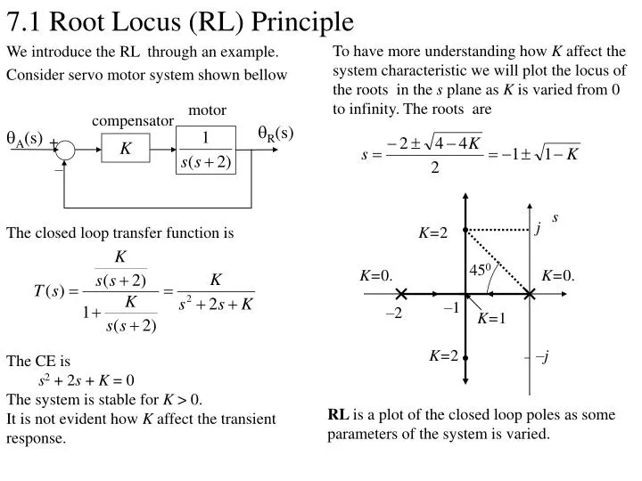
7.1 Root Locus (RL) Principle We introduce the RL through an example. Consider servo motor system shown bellow. motor. compensator. R (s). A (s). +. K. –. s. j. K= 2. 45 0. K= 0. . K= 0. . –1. –2. K= 1. K= 2. – j.

E N D
7.1 Root Locus (RL) Principle We introduce the RL through an example. Consider servo motor system shown bellow motor compensator R(s) A(s) + K – s j K=2 450 K=0. K=0. –1 –2 K=1 K=2 –j To have more understanding how K affect the system characteristic we will plot the locus of the roots in the s plane as K is varied from 0 to infinity. The roots are The closed loop transfer function is • The CE is • s2 + 2s + K = 0 • The system is stable for K > 0. • It is not evident how K affect the transient response. RL is a plot of the closed loop poles as some parameters of the system is varied.
7.1 Root Locus Principle s + K G(s) – H(s) The CE of this system is 1+KG(s)H(s)=0 (1) A value s1 is a point in the RL if and only if satisfies (1) for real 0<K<. For this system we call KG(s)H(s)the open loop function (OLF) Equation (1) can be written as K= –1/G(s)H(s) (2) Since G(s) and H(s) are generally complex and K is real then there are 2 condition must be met |G(s)H(s)|=1/|K| and (3) G(s)H(s) = r, r = ±1, ±3, ±5 … (4) We call (3) the magnitude criterion of the RL, and (4) the angle criterion. Any value s on the RL must meet both criterions. For 2nd order system the RL appears as a family of 2 paths or branches traced out by 2 roots of CE. We generally consider a system as in the following figure G(s) includes plant and compensator TF. The closed loop TF is
7.1 Root Locus Principle s1 s1- p2 s s1- z1 s1- p1 2 3 1 z1 p2 p1 To illustrate this criterion let us consider From the preceding discussion, it is seen that the condition of a point to be on the RL is that (all zero angles)– (all pole angles) = r where zero angle is the angle of s– zk and pole angle is the angle of s– pk . zk and pk are zero and pole of the OLF Calculating and plotting RL digitally is available and it is a convenient way to do it. However a good knowledge of the rule for plotting the RL will offer insight effect of changing parameter and adding poles and/or zeros in the design process. From mason gain formula, the CE is (s) = 1 + F(s) = 0 where F(s) is the OLF. Many design procedures are based on the OLF. Suppose that s1on the RL. Thus the angle condition becomes 1 – 2 –3= ± The locus of all points meet this condition forms the complete RL of the system
7.2 Root Locus Rules Since the TF is real function then its complex roots must exist in conjugate pairs, then RL is symmetrical with respect to the real axis Rule 1. RL is symmetrical with respect to the real axis With the zk and pk are zeros and poles of the OLF. The CE may be expressed as If the number of finite zeros < NP then the rest of zeros lies at infinity. If K but s remain finite then the branches of RL must approach the zeros of the OLF, else there must be zeros at infinity. This mean that RL finish at zeros of G(s)H(s). Rule 2. RL originates on the poles of G(s)H(s) for K=0 and terminates on the zeros of G(s)H(s) as K, including zeros at infinity. When there are zeros at infinity then the RL will extend to infinity as well. The asymptotes can be determined. If there is zeros at infinity then the OLF can be written as Therefore for K = 0 the roots of CE are simply the poles of OLF RL start at the poles of G(s)H(s). It is always that the number of zeros, NZ,, equalsthe number of poles, NP.
7.2 Root Locus Rules As s , the polynomial becomes Remember that the values of s must satisfy the CE 1-KG(s)H(s)= 0 regardless the value of s hence we have The asymptote intersect the real axis at hence we can write for large s s + Kbm=0 The angle of the roots are principal values of angle (asymptote angles) = r/r = ±1, ±3,… Where P is the finite poles and Z is the finite zeros
7.2 Root Locus Rules 7.3 Additional Techniques s - a p2 z1 p1 Rule 3 If OLF has zeros at infinity, the RL approach asymptote as K approach infinity. The asymptote intersect real axis at a with angle . Example. Consider the OLF Consider point a to the right of p1. The angle condition states that if a is on the RL then (all zero angles)– (all pole angles) = r. Since this not the case then any points on the real axis to the right of p1 are not on the RL. By the same argumentations we conclude that the points between p1 and p2 are on the RL, the points between p2 and z1 are not on the RL, the points to the left of z1 are on the RL. Rule 4 The RL includes all points to the left of an odd number of real critical frequencies (poles and zeros) There are 2 zeros at infinity, hence there are 2 asymptotes with angle ±900. The asymptote intersect the real axis at
7.3 Additional Techniques (2) Multiple roots on the real axis. If CE has multiple roots a on the real axis then we can write the characteristic polynomial as 1+KG(s)H(s) =(s-a)kQ(s) (1) Differentiating (1) with respect to s gives And (2) can be written as N(s)D’(s)- N’(s)D(s)=0 (3) The multiple points are breakaway points, they are points at which branches of RL leave or enter the real axis. Rule 5. The breakaway points on RL will appear among the roots of polynomial obtained either from (2) or (3). Since on the RL K = –1/ G(s)H(s) = –D(s)/N(s) we conclude that K’= N(s)D’(s)- N’(s)D(s)=0 Hence at breakaway points K is either maximum or minimum. For s =a it must be Hence the multiple roots a can be found by solving (2). Since G(s)H(s) is rational we can represent G(s)H(s)= N(s)/D(s)
7.3 Additional Techniques 1 s1 p1 3 p3 2 p2 Angle of Departure from Complex Poles Suppose the open loop poles are as shown in the figure below, and s1 is on the RL. For very small , 2=900, hence 1= 1800–900–3 Rule 6 Loci will depart from a pole pj (arrive at zj) at angle of d(a) where d = zi pi + r a = pi zi + r We are interested in finding the angle 1 when is very small. This is the angle of departure. From angle criterion we know that –1 –2 –3=1800
7.3 Additional Techniques -4/3 j -3 -2 -1 1 K=10 -j -0.132 p3 p2 p1 K=6 Example 1 We consider a system with OLF Routh-Hurwitz method can be used to find values of K for stability, this is found to be 6 < K< 10. (1) with 3 finite poles and 3 infinite zeros. Rule 2. The RL start from pole s =1, s = –2, and s = –3. Rule 3. The asymptote intersect the real axis at (1-2-3)/(3-0) = – 4/3, with angle ±600, and 1800. Rule 4. The RL occurs on the real axis for –2< s <1 and s<–3. As K is increased p1 and p3 move left, but p2 move right. Rule 5. Determine the breakaway point by differentiating (1) and set the result to zero. 3s2+8s+1=0 s1 = -0.132 and s2 = -2.54 (ignore s2)
7.3 Additional Techniques -2 -1 0.1 1 0.05 Example 3 Asimplified ship steering system modeled as a system of order 2 Example 2 The RL start from s =0 and s =0.1 and stop at s = . Two asymptotes at 900 intersect the real axis at s =0.05 The RL occurs on real axis for 0.1< s <1 Breakaway point at s = 0.05 The RL start from double pole s =0 and stop at zero s = 1 and s = One asymptote at 1800. The RL occurs on real axis for s < 1 Breakaway point at s = 0 and s = 2
7.3 Additional Techniques j0.4472 Ka=42 s =0.7 0.1 1 2 Example 4 The order-3 model of ship steering system is The CE is The Routh array is s3 1 0.2 s2 2.1 0.01Ka s1 (0.420. 01Ka)/2.1 Ka< 42 s0 0.01KaKa> 42 For stability 0<Ka<42. The auxiliary polynomial for Ka=42 is Qa = 2.1 s2 + 0.01(42) = 2.1 (s2 + 0.2) Setting Qa to zero we find s = ±j0.4472. At this point the system is oscillating with frequency = 0.4472 rad/s The RL start from poles s =0, s =0.1, & s =2 and stop at 3 zeros at s = 3 asymptotes intersect real axis at s =0.7 The real axis RL, for 0.1<s<0 and s<2 Breakaway point at s = 0.0494
7.3 Additional Techniques 1350 450 s =5.525 15.19 20 2 0 Example 5: The order-4 model of ship steering system is The RL start from poles s =0, s =0.1, s =2, & s =2 and stop at 4 zeros at s = 4 asymptotes intersect real axis at s =5.525. The real axis RL, for 0.1<s<0 and 20<s<2 Breakaway point at s = 0.0493, s = 15.19 For stability 0<Ka<38.03. For Ka=38.03 the system is oscillating with frequency 0.4254. j0.4254 Ka=38.03
7.3 Additional Techniques Table 1. Stabilities of the last 3 example Table 2. Poles of example 3, 4, and 5. The last 3 example illustrate RL construction and the reduction of order of system. From table 1 and 2 we see that for small Ka (=1) model of order 2 is adequate. For moderate Ka (= 20) model of order 3 is adequate. For large Ka (= 40) model of order 4 is required. Six rules for RL construction have been developed many additional rule are available for accurate RL graph, however we should use digital computer to draw accurate RL.
7.4 Additional RL properties p1 p3 p2 p2 p2 p2 p2 p1 p1 p1 p1 p1 p1 p1 p1 z1 z1 z1 p2 p2 p3 p3 Sketching RL relies on experiences, followings are some low order RL
7.4 Additional RL properties (1) (2) -2 -1 Example suppose we have OLF The CE can be written as D(s) + KN(s) =0 For a given K1we have D(s) + K1 N(s) =0 Suppose that K is increased by K2from K1then the CE becomes D(s) + (K1 + K2)N(s) =0 which can be expressed as The CE can be written as s2 + K(s+1)=0 For K=K1=2, we have s2+2s+2=(s+1)2+1=0 With roots s = 1±j. Thus the RL of OLF is the same with RL of (1) but start from 1±j. With respect to K2the locus appears to originate on roots as placed by letting K = K1but still terminates on the original zeros.
7.4 Additional RL properties (3) -2 -3 -4 -3 -2 -1 The RL of OLF The CE can be written as 1+ KG(s)H(s) =0 (1) Consider replacing s with s1 1+ KG(s-s1)H(s-s1) =0 (2) then for K0, (s-s1) = s0 satisfied (2). This is the efect of shifting all poles and zeros of the OLF by a constant amount s1. Example. The RL of OLF (3) is as shown below The last property is that a RL has symmetry at breakaway points. Suppose 4 branches come together at a common breakaway point, the the angle between 4 branches will be 3600/4=900. is as shown below
7.5 Other Configuration (2) compensator motor + – • Now (3) is the same form as (1) with • K= • and • G(s)H(s) = s/(s2+5) • In general the procedure is as follows • Write the CE in a polynomial of s • Grouped the terms that are multiplied by and that are not, that is we express • Dc(s) + Nc(s)=0 • Example • Let us design PI controller using RL. So far we plot RL of CE 1+ KG(s)H(s) =0 (1) by varying K from 0 to . Other system configuration should be converted to this form first. As an example let us vary from 0 to for the following CE or We rewrite the equation to yield and (3)
7.5 Other Configuration (1) (2) -0.5 0 The system CE is Now the RL is available, it is easier to specify the roots. Suppose we want critical damping condition then s =-0.5 and from (2) KP is Supposed that KI =1, and we want to vary KP and plot the RL. Eq. (1) becomes We have to rewrite this equation as The required PI compensator is then Gc(s) = 3.6 + 1/s and the design is complete The sketch of th RL is as follow j0.5 -j0.5