Download
1 / 70
700 likes | 710 Views
Lecture 6 Population Ecology. Eben Goodale College of Forestry, Guangxi University. So what did you think about sweaty T-shirts?. P = 0.023 R 2 = 0.09. 2.3 out of 100 times this result will be found by chance. X explains 9% of the Variance in Y. Where we are.

E N D
Lecture 6Population Ecology Eben Goodale College of Forestry, Guangxi University
So what did you think about sweaty T-shirts? P = 0.023 R2 = 0.09 2.3 out of 100 times this result will be found by chance. X explains 9% of the Variance in Y.
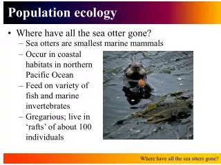
Where we are • Definition(定义) of ecology: interactions between organisms and their environment. • Started with physical environment • Then looked at how individual organisms balanced temperature, water, obtained energy.
Where we are • These organisms have adaptations to fit the environment. • We talked about evolution(进化论) and how natural selection produces adaptations. • Behaviors, too, are adaptations.
Where we are • So do individuals adapt? • No, this is a something that happens with a population(种群), as the individuals with the best adaptations survive and reproduce best. • We now move on to talking about populations and their properties: distribution(分布) (where they are), abundance(丰富) (how many), growth(生长) (how abundance changes), dynamics(动力学) (changes more complicated than growth).
Today’s outline:Population Ecology • Population density(密度)and dispersion • Life tables • Population growth • Exponential(指数) • Logistic(对数) • Population regulation • The situation with human population growth
Population Ecology Three main characteristics of a population: • Density(密度) • Dispersion(离差) • Demography(人口统计学)
Density • Density - Is the number of individuals per unit area or volume • What are the factors that • underlie this? Times Square • Birth • Death • Immigration(迁入) • Emigration(迁出) Abandoned town
Density • How do we measure it? • Census(人口普查)= everyone counted. • If can’t count all individuals, estimate by area, and extrapolation (推算). • An example of sampling (取样). If there are 12 kangaroo In 5 ha, how many in 5000 ha?
Density • How do we measure it? • But what if things are difficult to detect? • “Distance” analysis helps adjust for difference in detectability(检测能力) X
Density • How do we measure it? • But what if things are difficult to detect? • “Distance” analysis helps adjust for difference in detectability Probability of detection (检测概率) X Distance (m) 2 bird species (yellow and blue), blue loud; yellow soft and only heard nearby.
Density • How do we measure it? • Mark-recapture(标志重捕法): another example of sampling • capture some animals. • let them go. • recapture. • estimate population size.
Mark-Recapture m = # marked(被标记的) Assume that population mixes fully (假设人口 充分混合) x = marked recaptured(抓到中被标记的) n = total captured 2nd time(被抓到总数) N = estimated population size(推算出的总数) x/n = m/N N = (mn)/x
Exercise We are counted the population of the yellow-bellied motmot. 5 motmots were marked originally. Of a sample of 6 captured the second time, 1 was marked. How many motmots are there? A) 5 B) 7 C) 15 D) 30
Dispersion • Dispersion is the pattern of spacing among individuals • Random(随机分布), clumped(成群分布), or uniform(均匀分布). • Clumped and uniform interactions formed by interactions among individuals Competition Territorial behavior Facilitation(简易化) Grouping behavior Most common
Dispersion: an example from Western North America The creosote bush (Larrea tridentata) Medium age: competition amongst seedlings has ended clumping. Now random. Young: clumped because of seeds in groups. Old: Bushes get so big roots come into competition with others. End up evenly spaced.
Demography • Demography is the study of the vital statistics(动态变化) of a population • And how they change over time • Rates: • Birth rate • Death rate
Death rate can be seen through survivorship data • A life table is an age-specific summary of the survival pattern of a population
1000 100 Number of survivors (log scale) Females 10 Males 1 2 8 10 4 6 0 Age (years) Death rate can be seen through survivorship data Survival data can also expressed as a survivorship curve(生存曲线)
1,000 I 100 II Number of survivors (log scale) 10 III 1 100 50 0 Percentage of maximum life span Survivorship curves can be classified into three general types Types differ in the relative rates of juvenile and adult survival I: These kinds of organisms tend to live long and die of old age III: These kinds of organisms tend to die often as young Where are r (mouse) and K (elephant) strategies on this graph?
Birth rate can be seen through reproductive data A reproductive table describes the reproductive patterns of a population, by age group.
Calculating population growth through the life table What happens after year 5? Is this population growing? Because survivorship of older individuals is low, this mix of age classes is more typical of this population These original #s are a bit strange and atypical of this population
Calculating population growth through the life table This early instability caused by those weird initial numbers Otherwise, constant mortality and fecundity leads to constant λ (λ = population growth) log individuals Nt + 1 λ = Nt • time
Calculating population growth through the life table • Important to recognize: • Different mortality(死亡率), fecundity(生殖力) leads to different kinds of rate of growth • In nature, mortality and fecundity are not constant • This kind of life table shows time in step (t = 1,2,3 etc.) λ This early instability caused by those weird initial numbers Otherwise, constant mortality and fecundity leads to constant λ
λ is called the geometric rate of increase Nt+1 λ = Nt Rearrange Nt+ 1 = What’s Nt + 2? Nt+ 2 = Geometric growth(几何生长): calculated for pulsed reproduction(繁殖波动) (Nt) λ (Nt+ 1) λ When λ is ____, the population is stable. When λ is ____, the population is growing When λ is ____, the population is shrinking = ((Nt) λ) λ = Ntλ2 Generally Nt = Noλt
Larvae juveniles adults reproduction larvae juveniles adults reproduction Different kinds of reproduction: pulsed vs. continuous If all in one seasonal year, we consider this to be “pulsed”. Season 1, after which all adults die Season 2 On the other hand, if individuals of different ages are reproducing at once, as in humans, we consider it “continuous” reproduction(连续繁殖)
Now let’s talk about continuous reproduction r = per capita(人均) rate of increase of population (~ birth – death) death birth population Emigration (animals dispersing away) Immigration (animals dispersing in)
dN = (b – d) (N) dT Now let’s talk about continuous reproduction r = per capita rate of increase of population (~ birth – death) population death birth Assume “closed population” (no immigration, emigration), then Birth and death rates times the population present Differential equation(微分方程) = change in N over time
dN dN dN = (b – d) (N) dT dT dt = rmax (N) = r (N) rmax is the rate of growth for the species under ideal conditions and is by definition > 1 Continuous reproduction leads to exponential(指数) growth When r is ____, the population is stable. When r is ____, the population is growing When r is ____, the population is shrinking Can we solve for Nt, just as we did for geometric growth?
dN dt dN Integrate both sides = r (dt) N = r (N) ln (Nt/N0) = rt Where No is the population at time=0 And Nt is the population at time=t = er(t) Nt/N0 The exponential growth equation e = 2.718 Nt = Noer(t) Nt = Noλt Notice the similarity Continuous reproduction leads to exponential growth
Nt = Noer(t) Nt = Noer(t) Nt = Noert Nt = Noert Exponential growth What happens when r = 0? Nt = Noe(0) Nt = N0 What happens when r > 0 … let’s say it’s 1…, and let’s look at t = 1. N1 = Noe(1) N1 = No(2.718) What happens when r < 0 … let’s say it’s -1…, and let’s look at t = 1. N1 = Noe(.95) Nt = No(.368)
Nt = Noert Exponential growth …let’s solve some problems How many duckweeds in cm2 after 4 days? Original amount = 10 per cm2 r = .20 duckweeds per day per cm2 N4 = (10)(2.718^.8) 22 per cm2
ln(Nt/No) ln(426/40) r = r = t 2 Nt = Noert Exponential growth …let’s solve some problems Solve for r Pheasants on Protection Island went from 40 to 426 individuals In 2 years …. What’s r? r = 1.18
Doubling time • Question: For a given growth rate r, how long before the population doubles? • Recall Nt = N0 * ert, now we are asking, “what is the value of t such that Nt = 2N0? • 2N0 = N0 * ert • 2N0 / N0 = ert • 2 = ert • ln(2) = rt • (ln2)/r = t (the natural log of 2 = 0.693147…)
Exercise If the human population is growing at a rate of 1.5% a year, the doubling(加倍) time is • 13 years • 46 years • 102 years • 105 years Hint: First solve Nt = Noert For t = 1, and find r Then use (ln2)/r = t To find doubling time This is the same equation we use for compounding interest. A savings account that receives 1.5% annual interest will double in 46 years.
Exponential population growth • Let’s now explore what happens when population growth is highest; that is, when conditions are ideal: dN/dt = rmaxN • Let’s plot population size vs. time: As population growth (dN/dt) is dependent on N, the size of the population, it keeps escalating as N gets bigger
Exponential population growth:does this really happen? • This happens in rare situations, like when bacteria are just started to let multiply on an agar plate, or a population that was threatened is protected: In other words, when there’s no limitingfactors (限制因子) Elephants after hunting stopped
Logisitic growth(对数增长) • Exponential growth • Cannot be sustained(持续) for long in any population • (Otherwise we would be knee deep in fruit flies, or worse!) • A more realistic population model • Limits growth by incorporating carrying capacity(承载力) Carrying capacity = maximum population size that a particular environment can sustain
Deriving the logistic equation • We want an equation in which population growth decreases as density gets higher
Deriving the logistic equation Line: r = mN + b Plug in slope and intercept
Deriving the logistic equation dN/dt = rmaxN
dN dt = rmax (N) The logistic equation N (1 - ) K What is K? K is the “carrying capacity” When N > K, what is dN/dt? When N = K, what is dN/dt? When N < K, what is dN/dt?
The logistic equation dN dt N What does this graph look like?
The logistic equation OK, now say that you are managing a aquaculture farm, Raising fish. How many fish would you want to have?
Exercise You’re a fish farmer and you have found out that the carrying capacity for the fish in your tanks is 3000 fish. At how many fish should you keep the population so that your annual harvest is best? • 1,000 • 1,500 • 3,000 • 6,000
The Logistic Model and Real Populations But other organisms shown a trend to overshoot(超过) the carrying capacity, and then had back down to it, settling up an oscillating(震荡的) pattern…. Indicates that there’s some time-lag 时间间隔)before the effects of the carrying capacity are felt.
Some assumptions(假设) of the logistic growth model • K always stays the same • Every additional individual has the same effect on the resources. • There is no time lag between reaching K and feeling the effects of K A famous prediction of human Population growth in the 1920’s (dashes; real data is circles)
Exercise In the 1920’s, scientists used the logistic equation to estimate population growth. However, their estimates were much too low. What mistake did they make? • They miscalculated r. • They forgot that the effects of K had a time lag. • They didn’t realize K would change Estimated population was the curved line; actual data the circles
Today’s outline:Population Ecology • Population density and dispersion • Life tables(生命统计表) • Population growth • Exponential • Logistic • Population regulation • The situation with human population growth