Download
1 / 29
290 likes | 292 Views
This document presents the results of the intercalibration process in Alpine rivers for the assessment of macro zoobenthos. It discusses different options for the intercalibration process and provides guidance on the selection of reference sites and quality criteria. The document also includes the calculation methods for the Intercalibration Common Metric Index (ICMi) and presents the results of the qualitative and quantitative ICM. Overall, the ICM is found to be a suitable instrument for comparison and the boundaries of the status classes are within an acceptable range, although slight adjustments may be needed in some cases. The document concludes that data quality and quantity will improve in the future with monitoring programs, enhancing the scientific accuracy of intercalibration.

E N D
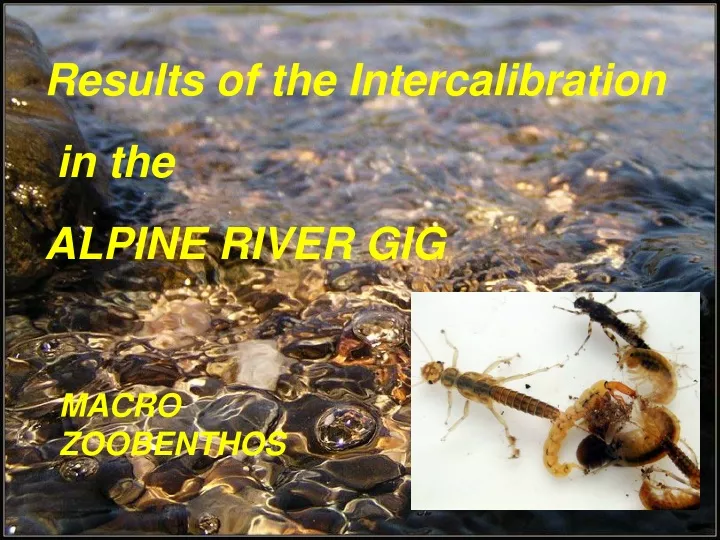
Results of the Intercalibration in the ALPINE RIVER GIG MACRO ZOOBENTHOS
Introduction: Common Intercalibration Type: Alpine Rivers From: ECOSTAT WG 2.A, 2004: Overview of common Intercalibration types
Introduction: The 3 Options for the Intercalibration Process HYBRID OPTION • Option 1: Common WFD Assessment method • Option 2:Use of a common metric(s) method identified specifically for the purposes of the intercalibration exercise • Option 3:Direct comparison of national methods at intercalibration sites From: ECOSTAT WG 2.A, 2004: Guidance on the Intercalibration Process
Introduction: The 3 Options for the Intercalibration Process • HYBRID OPTION • establish boundary values with national assessment methods (as in Option 3) • subsequent comparison of boundary values with common metrics method (as in Option 2). • Comparison: ICMialpine (qualitative, quantitative) • Harmonisation: Median boundary value
Introduction: METHODS ICMi - qualitativeAlpine GIG
Introduction: METHODS ICMi - quantitativeAlpine GIG Calculation of ICM: weighted sum
Reference conditions • The selection of reference sites was based on common criteria (see Annex B). • The reference value was calculated by using the median of reference sites • Number of sites/coutry:
Introduction: Quality checks ICMi:Minimum Quality Criteria • minimum : 20 sites covering widest range of quality classes • reference state compliant to the REFCOND guidance • Pearson R²: national index vs. ICMi: >=0.64 (at a=0,05)
Introduction: METHODS ICMi:Quality Criteria
Introduction: METHODS ICMi:Standardization of Calculation • 4 metrics (qual. ICM) / 6 metrics (quant. ICM) • reference value: median of reference sites • EQR for every value = value / reference • ICM: average (qual.) / weighed sum (quant.) • Regression of EQRnational vs EQRICM • Regression formula, R² • Transformation of national EQR boundary values into EQR ICM - values
Introduction: METHODS Key metrics and ICMi: Example SPAIN
Results ICM – causes of variation: • ICM is a simplifying approach • linear relationship is a simplification • less accuracy / confidence than nat. methods • typology • ICM typology coarse – more simple than nat. types • “problems” with min. qual. criteria • new methods – lack of data and experience • quality of our streams is “to good” conclusion: “accepted variation” of boundary values instead of fixed value is necessary
Acceptable range of variation • As a consequence the Alpine GIG suggests to use an „acceptable range of variation“ rather than a fixed value alone. • As value for this „acceptable range of variation“ the GIG proposes ¼ of the median status class width of the participating member states.
Results Of the ICM Intercalibration procedure QUALITATIVE ICM
Results Results R-A1:calcareous type
Results Discriminatory power of the ICMi class boundaries National ranges of status classes expressed with ICMi values. Boxplots: 25th percentile – median - 75th percentile. Whiskers above and below the box indicate the 90th and 10th percentiles.
Results Discriminatory power of the ICMi class boundaries National ranges of status classes expressed with ICMi values. Boxplots: 25th percentile – median - 75th percentile. Whiskers above and below the box indicate the 90th and 10th percentiles.
Results Of the ICM Intercalibration procedure QUANTITATIVE ICM
Correlation ICMiqualitative - ICMiquantitative for member states with available quantitative data.
CONCLUSION Conclusion • ICM is a proper instrument for comparison • Quantitative and qualitative ICM show comparable results • “accepted range of variation” is necessary due to several sources of variation • Boundaries seem to be in an acceptable range, especially for the type R-A2 • In some cases slight changes of national boundary values are probably necessary (IT, ES) • Data quality and quantity will enhance in future with monitoring programmes – increasing the scientific accuracy of the intercalibration
Alpine GIG people (Homo alpinus var. Intercalibrensis) Thanks to all of you!!!
Background of this proposal: The results of the assessment methods are subject to several sources of variation. Thus the status assessment is somehow more significant in the middle of a status class than compared to the transitional zone to the neighbouring status classes. This “insecure” zone of assessment is assumed to be ¼ of the status class width (more detailed estimates of accuracy and precision is lacking in most countries at the moment).
As an alternative approach the bands of “accepted variation” were also calculated as median confidence limits of all member states • From the statistical point of view this approach does not seem to be appropriate, as the confidence limits are decreasing with increasing data quality, but the sources of variation if the results are still present