Download
1 / 43
430 likes | 515 Views
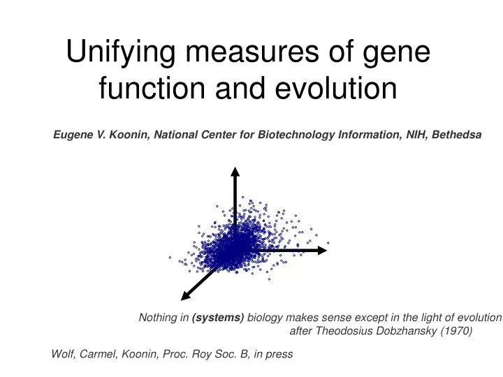
Unifying measures of gene function and evolution. Eugene V. Koonin, National Center for Biotechnology Information, NIH, Bethedsa. Nothing in (systems) biology makes sense except in the light of evolution after Theodosius Dobzhansky (1970). Wolf, Carmel, Koonin, Proc. Roy Soc. B, in press.

E N D
Unifying measures of gene function and evolution Eugene V. Koonin, National Center for Biotechnology Information, NIH, Bethedsa Nothing in (systems) biology makes sense except in the light of evolution after Theodosius Dobzhansky (1970) Wolf, Carmel, Koonin, Proc. Roy Soc. B, in press
Systems Biology and Evolution With the advent of OMICS data… The game of correlations began…
Evolutionary systems biology: • In principle, we address the classical problem: the relationship between the (largely neutral?) evolution of the genome and the (largely adaptive) evolution of the phenotype • In practice, the progress of genomics + other OMICS allows us to measure, on whole-genome scale, the effects of all kinds of molecular phenotypic characteristics (expression level, protein-protein interactions etc etc) on evolutionary rates – this typically yields weak, even if significant, correlations • Can we synthesize these measurements to produce a coherent picture of the links between phenomic and genomic evolution?
The Cautionary Tale "It was six men of Indostan / To learning much inclined, Who went to see the Elephant / (Though all of them were blind), That each by observation / Might satisfy his mind " (J.G. Saxe)
The Cautionary Tail "…each was partly in the right / And all were in the wrong" (J.G. Saxe)
Different Faces of the Hypercube? Pairwise correlations Synthesis
"fair world" model "unfair world" model Analysis of Multidimensional Data
Analysis of Multidimensional Data PC1 PC3 PC2 Principal Components Analysis (PCA) introduces a new orthogonal coordinate system where axes are ranked by the fraction of original variance accounted for.
PCA • PCA takes a set of variables and defines new variables that are linear combinations of the initial variables. • PCA expects the variables you enter to be correlated (as is the case in the correlation game of Systems Biology). • PCA returns new, uncorrelated variables, the principal components or axes, that summarize the information contained in the original full set of variables. • PCA does not test any hypotheses or predict values for dependent variables; it is more of an exploratory technique. • The data entered represent a cloud of points, in n-space. • The cloud is, typically, longer in one direction than another, and that longest dimension is where the points are the most different; that's where PCA draws a line called the first principal component. • The first principal component is guaranteed to be the line that places your sample points the farthest apart from each other, in that way, PCA "extracts the most variance" from your data. This process is repeated to get multiple components, or axes.
The Data Set: KOGs • Ideally, we would like to obtain and synthesize the data on individual genes in precise space-time coordinates (e.g., instant evolutionary rates) • However: • some of the variables are not easily measurable (if defined at all) for genes in extant species [e.g. rate of evolution]; • other variables are measurable in principle but, in practice, are • available only for a few species [e.g., expression level] • much of the data are inherently noisy, either due to technical problems or true biological variation [e.g. fitness effect of gene disruption]. • Thus, we analyze orthologous protein sets, using the proteins from different species to derive complementary data and smooth out variations in other. • Practically, this means using the KOG dataset (with additions): 10058 KOGs from 15 species (Koonin et al. 2004, Genome Biol).
Arath Orysa Dicdi Enccu Maggr Neucr Schpo Sacce Canal Caeel Caebr Drome Cioin 100 Myr Homsa Musmu The Data Set: KOGs Original KOGs for some species, "index orthologs" for other. 10058 KOGs altogether
At Ce Dm Hs Sc Sp Ec Gene loss Variables: Gene Loss Propensity for Gene Loss (PGL), introduced by Krylov et al. (Genome Res.13, 2229-2235, 2003). Computed from KOG phyletic pattern. Originally an empirical measure (Dollo parsimony reconstruction of events; ratio of branch lengths). In this work – employs an Expectation Maximization algorithm.
Variables: Gene Duplication Number of Paralogs, average number observed for a given KOG. Example: KOG0417 (Ubiquitin-protein ligase) and KOG0424 (Ubiquitin-protein ligase).
Variables: Evolution Rate Select a taxon Build an alignment (MUSCLE); Compute distance matrix (PAML); Select minimum distance between members of the two subtrees of the group. Ascomycota: Sordariomycetes vs. Yeasts
Variables: Expression Level Expression Level data for S. cerevisiae, D. melanogaster and H. sapiens were downloaded from UCSC Table Browser (hgFixed). Organism Table No. exp. No. prob. No. KOGs Sacce yeastChoCellCycle 17 6602 3030 Drome arbFlyLifeAll 162 4921 2617 Homsa gnfHumanAtlas2All 158 10197 3872 Standardized (=0; =1) log values; median expression level among paralogs was used to represent a KOG.
Variables: Interactions Protein Protein and Genetic Interactions (PPI and GI) data for S. cerevisiae, C. elegans and D. melanogaster were downloaded from GRID Web site. Median number of interaction partners among paralogs was used to represent a KOG.
Variables: Lethality Lethality of Gene Knockout data for S. cerevisiae were downloaded from MIPS FTP site (0/1 values). Embryonic Lethality of RNAi Interference data for C. elegans were taken from Kamath et al., 2003 (0/1 values).
Missing Data Total: 38 variables in 10058 KOGs – lots of missing data. Complete data (all 38 variabless available): 23 KOGs – too few. Combined data: 7 variables, 1482 KOGs with complete data; 4124 with at most one missing point; 3912 KOGs after removal of outliers. Example: evolution rate. At.Os Sc.Ca Mg.Nc Hs.Mm. Pl.MF KOG0009 - 0.168 0.300 - 0.405 KOG0010 0.671 1.252 0.606 0.087 1.492 KOG0011 0.905 1.698 0.428 0.073 1.547 KOG0012 - 2.238 0.665 0.244 - KOG0013 0.355 - - 0.014 1.343 KOG0014 1.913 4.041 - 0.126 2.840 KOG0015 - 2.286 0.400 0.027 - KOG0016 - - 0.506 0.380 - 0.667 1.864 0.521 0.075 1.910 At.Os Sc.Ca Mg.Nc Hs.Mm. Pl.MF - 0.090 0.575 - 0.212 1.006 0.672 1.162 1.166 0.781 1.358 0.911 0.821 0.984 0.810 - 1.201 1.275 3.275 - 0.532 - - 0.181 0.703 2.869 2.168 - 1.692 1.487 - 1.227 0.767 0.365 - - - 0.970 5.087 - Average 0.293 0.957 0.977 1.917 0.472 2.054 0.786 3.028
Variables • Phenotypic • EL – expression level • PPI – protein-protein interactions • GI – genetic interactions • KE – knockout effect • NP – number of paralogs • Evolutionary • ER – (sequence) evolution rate • PGL – propensity for gene loss
The correlations NP PPI GI PGL ER EL KE NP - PPI 0.057 - GI 0.060 0.034 - PGL 0.000 -0.125 -0.019 - ER -0.070 -0.2000.034 0.141 - EL 0.129 0.199-0.050 -0.099 -0.277 - KE 0.027 0.234-0.048 -0.181 -0.1550.188 -
"phenotypic" variables "bigger is better" "evolutionary" variables "slow is good, fast is bad" Two Tiers of Variables Observation on the pattern of pairwise relationships in the data: "phenotypic" and "evolutionary" variables behave differently.
"phenotypic" variables positive "evolutionary" variables negative positive Two Tiers of Variables Observation on the pattern of pairwise relationships in the data: "phenotypic" and "evolutionary" variables behave differently.
non-essential (almost by definition) low-expressed relatively fast-evolving The correlations NP PPI GI PGL ER EL KE NP - PPI 0.057 - GI 0.060 0.034 - PGL 0.000 -0.125 -0.019 - ER -0.070 -0.2000.034 0.141 - EL 0.129 0.199-0.050 -0.099 -0.277 - KE 0.027 0.234-0.048 -0.181 -0.1550.188 -
Sphericity PCA of the Data Space PC.1 PC.2 PC.3 NP 0.17 0.69 0.44 PPI 0.46 0 -0.17 GI 0 0.67 -0.54 PGL -0.33 0 0.51 ER -0.47 0 -0.20 EL 0.48 0 0.36 KE 0.45 -0.27 -0.21 ----------------------------------------- % var. 25.0 15.3 14.5
PCA of the Data Space PC2 PC1
PCA of the Data Space PC3 PC2
PC1 – Gene’s “status" PC2 "accessory" "important" PC1
PC2 – "Adaptability" "flexible" PC2 "rigid" PC1
Skew ~0 Skew >0 Status - LO Status - HI PC2 PC2 LO HI p-value LO HI p-value S. cerevisiae 0.29 0.29 1x100 0.32 0.44 3x10⁻³ D. melanogaster 1.82 1.84 4x10⁻¹ 1.82 1.90 7x10⁻² H. sapiens 1.75 1.94 7x10⁻⁴ 1.87 2.12 <1x10-20 Omnibus test 1x10⁻² <1x10-20 PC2 and Expression Profile Skew
PC3 – "Reactivity" PC3 PC2
Skew ~0 Skew >0 Status - LO Status - HI PC3 PC3 LO HI p-value LO HI p-value S. cerevisiae 0.26 0.31 3x10⁻¹ 0.22 0.50 <1x10-20 D. melanogaster 1.77 1.88 6x10⁻² 1.86 1.85 9x10⁻¹ H. sapiens 1.80 1.94 3x10⁻⁴ 1.86 2.13 <1x10-20 Omnibus test 4x10⁻⁴ <1x10-20 PC3 and Expression Profile Skew
"STATUS" "ADAPTABILITY" "REACTIVITY" "phenotypic" variables "evolutionary" variables Relationships Between Variables
Status and Adaptability of Genes Classification of KOGs into 4 major categories
Status and Adaptability of Genes Status INF CELL Adaptability MET Reactivity UNKN Classification of KOGs into 4 major categories
Status and Adaptability of Genes Cytoplasmic and Mitochondrial ribosomal proteins
Status and Adaptability of Genes Vacuolar ATPase and Vacuolar Sorting proteins
Status and Adaptability of Genes Replication Licensing Complex and Histones
Status and Adaptability of Genes Core Cluster (spliceosome and mRNA cleavage-polyadenylation complex) RNA processing and modification
Adaptability and Reactivity of Genes carbohydrate transport and metabolism translation and ribosome replication, RNA processing and modification signal transduction
Conclusions • Three composite, independent variables – "status","adaptability"and"reactivity" – dominate the multidimensional data space of quantitative genomics. • The notion of status provides biologically relevant null hypotheses regarding the connections between various measures. • Breaks in the pattern possibly indicate something nontrivial (targets for further investigation). • Functional groups of genes show distinctive patterns of status, adaptability, and reactivity
Co-Authors Liran Carmel Eugene Koonin Yuri Wolf