Download
1 / 16
160 likes | 166 Views
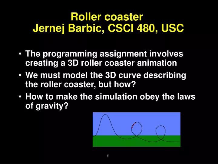
Roller coaster Jernej Barbic, CSCI 480, USC. The programming assignment involves creating a 3D roller coaster animation We must model the 3D curve describing the roller coaster, but how? How to make the simulation obey the laws of gravity?.

E N D
Roller coaster Jernej Barbic, CSCI 480, USC • The programming assignment involves creating a 3D roller coaster animation • We must model the 3D curve describing the roller coaster, but how? • How to make the simulation obey the laws of gravity?
Back to the physics of the roller-coaster:mass point moving on a spline frictionless model, with gravity P • Velocity vector always pointsin the tangential directionof the curve v spline
Mass point on a spline (contd.)frictionless model, with gravity • Our assumption is : no friction among the point and the spline • Use the conservation of energy law to get the current velocity • Wkin + Wpot = const = m * g * hmax • hmax reached when |v|=0 • Wkin = kinetic energy = 1/2 * m * |v|2 • Wpot = potential energy = m * g * h • h = the current z-coordinate of the mass point • g = acceleration of gravity = 9.81 ms-2 • m = mass of the mass point
Mass point on a spline (contd.)frictionless model, with gravity • Given current h, we can always compute the corresponding |v|:
Mass point motion* • Assume we know the initial position of a mass point, and velocity v=v(t) • Velocity is a 3-dim vector • Problem: compute the position of the point at an arbitrary time t1 • Has to integrate velocity over time: • x, v are vectors
Mass point motion (contd.)* • Usually, cannot compute the integral symbolically • Numerical integration necessary • Standard numerical integration routines can be used(i.e. Simpson, Trapezoid, etc.) • Integrate each of the coordinates x,y,z separately • This is a general approach • For motion on a spline, use arclength parameterization approach instead
Arclength Parameterization • There are an infinite number of parameterizations of a given curve. Slow, fast, speed continuous or discontinuous, clockwise (CW) or CCW… • A special one: arc-length-parameterization: u=s is arc length. We care about these for animation. u=0s=0 need control over velocity along the curve for animation u=1s=7.4 u=0.8s=3.7 • Problem: parameterizations usually aren’t arc-length • How to transform parameterization to an arc-length parameterization?
Arclength Parameterization (contd.) • Assume a general parameterization p=p(u) • p(u) = [x(u), y(u), z(u)]T • arclength parameter s=s(u) is the distance from p(0) to p(u) along the curve • Distance increases monotonically, hence s=s(u) is a monotonically increasing function • It follows from Pitagora’s law that
Arclength parameter s • The integral for s(u) usually cannot be evaluated analytically, not even for cubic splines (simple polynomials) • Has to evaluate the integral numerically • Simpson’s integration rule (next slide) • Piecewise polynomial definition of the spline means we have to break the integral over individual spline pieces • For a fixed spline, can pre-compute function s=s(u) for certain values of u and store it into an array • For the next slides, we will assume we have a routine, which computes s(u), given a value of u
Simpson integration rule • a = x1, b=xn, h=(b-a)/(n-1) • h = x2k+1-x2k = x2k-x2k-1 = independent of k • n > 3 corresponds to the number of intervals • formula exact for a cubic polynomial • n MUST be odd • Must be able to evaluate the function at the points x2k-1,x2k,x2k+1 • Alternative to Simpson: Trapeziod rule • Less accurate: Error is O(h3) • Simpler to compute than Simpson
Inverse u=u(s) • Inverse problem: Given arclength s, determine the original parameter u • Since s=s(u) is monotonically increasing, so is u=u(s) • Useful (necessary) for animating motion along the curve • Since u=u(t) can only be computed numerically, there is no exact formula for u=u(s)
Computing inverse u=u(s) • Given arclength s, we can use bisection to determine the corresponding u • Can compute (using Simpson’s rule) the function s=s(u) in the forward direction Arclength parameter s=s(u) s we know Original parameter u we look for
Computing inverse u=u(s) • Must have initial guess for the interval containing u • Bisection(umin,umax,s) • /* umin = min value of u • umax = max value of u; umin <= u <= umax • s = target value */ • Forever // but not really forever • { • u = (umin + umax) / 2; // u = candidate for solution • If |s(u)-s| < epsilon • Return u; • If s(u) > s // u too big, jump into left interval • umax = u; • Else // t too small, jump into right interval • umin = u; • }
Simulating mass point on a spline • Assume we know the size of the current velocity vector |v| of a mass particle on the spline at a given moment in time t • Can obtain this using the laws of physics, as shown before • Notation: • u = original parameterization • t = time • s = natural parameterization (i.e. arclength parameterization) • We keep current u, t and s in three separate variables • How to compute the next position of the particle?
Simulating mass point on a spline • Time step t • We have: s = |v| * t and s = s + s . • We want the new value of u, so that can compute new point location • Therefore:We know s, need to determine uHere we use the bisection routine to compute u=u(s).
Mass point simulation • Assume we have a 32-piece spline, with a general parameterization of u[0,31] • MassPoint(tmax) // tmax = final time • /* assume initially, we have t=0 and point is located at u=0 */ • u = 0; • s = 0; • t = 0; • While t < tmax • { • Assert u < 31; // if not, end of spline reached • Determine current velocity |v| using physics; • s = s + |v| * t; // compute new arclength • u = Bisection(u,u + delta,s); // solve for t • p = p(u); // p = new mass point location • Do some stuff with p, i.e. render point location, etc. • t = t + t; // proceed to next time step • }