Download
1 / 15
150 likes | 155 Views
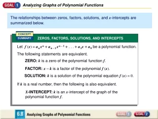
6.8 Analyzing Graphs of Polynomial Functions. Analyzing Graphs of Polynomial Functions. CONCEPT. SUMMARY. The relationships between zeros, factors, solutions, and x -intercepts are summarized below. ZEROS, FACTORS, SOLUTIONS, AND INTERCEPTS.

E N D
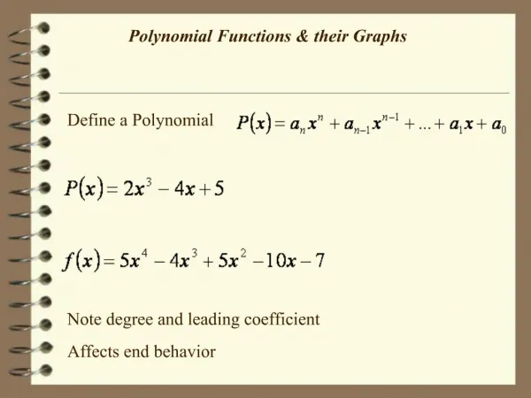
Analyzing Graphs of Polynomial Functions CONCEPT SUMMARY The relationships between zeros, factors, solutions, and x-intercepts are summarized below. ZEROS, FACTORS, SOLUTIONS, AND INTERCEPTS Let f (x) = anxn+an – 1xn – 1+ . . . +a1x+a0 be a polynomial function. The following statements are equivalent. ZERO:k is a zero of the polynomial function f. FACTOR:x–k is a factor of the polynomial f (x). SOLUTION:k is a solution of the polynomial equation f (x) = 0. If k is a real number, then the following is also equivalent. X-INTERCEPT:k is an x-intercept of the graph of the polynomial function f.
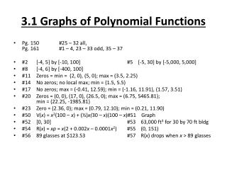
Using x-Intercepts to Graph a Polynomial Function 1 4 (x+ 2)(x– 1)2. Graph the function f(x) = x –4 –3 –1 0 2 3 1 2 1 2 y –4 1 1 5 –12 Because f (x) has three linear factors of the form x – k and a constant factor of , it is a cubic function with a positive leading coefficient. 1 4 SOLUTION Plot x-intercepts. Since x + 2 and x – 1 are factors of f (x), –2 and 1 are the x-intercepts of the graph of f. Plot the points (–2, 0) and (1, 0). Plot pointsbetween and beyond the x-intercepts. Determinethe end behavior of the graph.
Using x-intercepts to Graph a Polynomial Function 1 4 (x+ 2)(x– 1)2. Graph the function Therefore, and f(x) f(x) as x as x – – Drawthe graph so it passes through the points you plotted and has the appropriate end behavior.
Remember End-Behavior EVEN DEGREES: • Positive L.C, Even Degree (both up) • Positive L.C, Odd Degree (Right up, Left down) • Negative L.C., Even Degree (both point down) • Negative L.C., Odd Degree (Left up, Right down) UP – UP (POSITIVE) DOWN – DOWN (NEGATIVE) ODD DEGREES: RISE TO THE RIGHT (POSITIVE) FALLS TO THE RIGHT (NEGATIVE)
Graph the Function Plot the intercepts. Make a table and plot some points. What are the end behaviors? What kind of function is it?
Graph the Function Plot your zeros. Multiply the factors together to tell you about end behavior
Analyzing Polynomial Graphs TURNING POINTS Another important characteristic of graphs of polynomial functions is that they have turning points corresponding to local maximum and minimum values. The y-coordinate of a turning point is a local maximum of the function if the point is higher than all nearby points. The y-coordinate of a turning point is a local minimum of the function if the point is lower than all nearby points. TURNING POINTS OF POLYNOMIAL FUNCTIONS The graph of every polynomial function of degree n has at most n–1 turning points. Moreover, if a polynomial function has n distinct real zeros, then its graph has exactlyn– 1 turning points.
Estimate the coordinates of the turning point. Is it a local minimum or a local maximum?
What degree is the function? Click on the link… • Polynomial Function Graphs • Use the website to determine what the coefficients of the terms do.
Using Polynomial Functions in Real Life You are designing an open box to be made of a piece of cardboard that is 10 inches by 15 inches. The box will be formed by making the cuts shown in the diagram and folding up the sides so that the flaps are square. You want the box to have the greatest volume possible. How long should you make the cuts? What is the maximum volume? What will the dimensions of the finished box be?
Using Polynomial Functions in Real Life You are designing an open box to be made of a piece of cardboard that is 10 inches by 15 inches. The box will be formed by making the cuts shown in the diagram and folding up the sides so that the flaps are square. You want the box to have the greatest volume possible. How long should you make the cuts? What is the maximum volume? What will the dimensions of the finished box be? SOLUTION Verbal Model Volume= Width Length Height Volume = V (cubic inches) Labels (inches) Width = 10 – 2x (inches) Length = 15 – 2x (inches) Height = x …
Using Polynomial Functions in Real Life You are designing an open box to be made of a piece of cardboard that is 10 inches by 15 inches. The box will be formed by making the cuts shown in the diagram and folding up the sides so that the flaps are square. You want the box to have the greatest volume possible. How long should you make the cuts? What is the maximum volume? What will the dimensions of the finished box be? … Algebraic Model V = (10 – 2x)(15 – 2x)x = (4x2– 50x+ 150)x = 4x3– 50x2+ 150x
Using Polynomial Functions in Real Life You should make the cuts approximately 2 inches long. The maximum volume is about 132 cubic inches. The dimensions of the box with this volume will be x = 2 inches by 10 – 2x = 6 inches by 5 – 2x = 11 inches. You are designing an open box to be made of a piece of cardboard that is 10 inches by 15 inches. The box will be formed by making the cuts shown in the diagram and folding up the sides so that the flaps are square. You want the box to have the greatest volume possible. How long should you make the cuts? What is the maximum volume? What will the dimensions of the finished box be? To find the maximum volume, graph the volume function. Consider only the interval 0 < x < 5 because this describes the physical restraints on the size of the flaps. From the graph, you can see that the maximum volume is about 132 and occurs when x1.96.