Download
1 / 17
170 likes | 246 Views
Probabilistic Modeling of Molecular Evolution Using Excel, AgentSheets , and R. Jeff Krause (Shodor ). Biological Sequence Space is Discrete. Probability theory is crucial to understanding sequences Furthermore, metrics and algorithms for analyzing sequences are statistical.

E N D
Probabilistic Modeling of Molecular Evolution Using Excel, AgentSheets, and R Jeff Krause (Shodor)
Biological Sequence Space is Discrete • Probability theory is crucial to understanding sequences • Furthermore, metrics and algorithms for analyzing sequences are statistical
Sequence Comparison: Similarity/Distance CAGTTAGCTC CATTAAGCTC Proportional distance (p) = # of differences in aligned positions p = 2 differences in 10 positions p = 0.2
Character Evolution in Biological Sequences CAGTTAGCTC ||+|+||+|| CATTCAGATC ||||+||+|| CATTAAGCTC
Probabilistic Modeling of Sequence Evolution • During replication (and recombination), errors occur • Substitution, insertion, deletion, inversion, translocation, … • Different types of errors have different chances of occurring, but they can all be considered to happen randomly • To develop models we need data to indicate how often each type of error occurs • Use observed frequencies and our understanding of the mechanism of error occurrence to estimate probabilities of errors
Stochastic Modeling of Sequences … and More • Yesterday we talked about dynamic modeling with difference equations and rates of change • Instead of thinking in terms of rate or proportion per unit time, we could think in terms of probability of occurring within a time-step • So all of our dynamic models yesterday could be modeled probabilistically
Probability Terms – Part I • Trial – A single occurrence of a random process (e.g. a single coin toss, or roll of a die) • Outcome – The result of a trial (e.g. “heads” or “tails”) • Probability – The chance of a random outcome occurring (e.g. p(heads)=0.5, p(3)=1/6) • Frequency – The number of occurrences of an outcome • Relative frequency – Number of occurrences of an outcome divided by the total number of trials
Probability Terms – Part II • Event – A grouping of multiple outcomes (e.g. “roll an odd number”, “roll less than 5”) • Independent – The probability of an outcome is not influenced by the outcomes of previous trials • Multiplication rule – The probability that two independent outcomes will occur is the product of their individual probabilities (e.g. “toss two heads”, “roll is odd and <= 4)
Coin Toss • Create an Excel worksheet that conducts 10, 100, or 1000 trials of a coin toss • Tally the frequency of heads for each number of trials • Is it a fair coin? How do you know. • Variation in composition vs sample size • Degree of variation with sample size (range or difference between (max – min) 3 of heads • Probably smaller with small sample sizes since sample size limits range • Larger sample size makes variation across larger range possible • Proportional variation vs sample size • Much larger for small samples since small differences in observed frequency have larger effect when divided by small denominator of small sample • Probability of a given sequence of outcomes – multiplication rule multiple independent events • Permutations – 2n different n-length sequences • Probability of event specifying sequence composition – enumerate permutations and sum probabilities of events matching criteria, this is the addition rule
Die Roll • Is it a fair die? How do you know? • Event probabilities for single trial • p(odd), p(odd and < 5) • Event probabilities for two trial events • p(2,5), p(2,5 in any order), p(sum is 7) – (use plop-it) • Union and intersection – explore addition rule and mutual exclusive, as well as multiplication rule and independence • Probability of a given sequence of length n = 6n
Probability Terms – Part III • Union – The event that either or both of two events will occur on a trial (e.g. the union of “odd” and “>4” is “1,3,5,6”) • Mutually exclusive – Two events are mutually exclusive if they can’t occur simultaneously (e.g. “roll an even number” and “roll an odd number”) • Addition rule – The probability of an event consisting of mutually exclusive outcomes is the sum of the probabilities of the outcomes (e.g. p(heads,tails) = p(heads) + p(tails) • Complement – The complement to any event includes all possible outcomes not in the event (e.g. “not heads”, “not 5”). The probability of the complement is ( 1 – the probability of the event) • Exhaustive – The set of all possible outcome, the probability must sum to 1
Molecular Evolution and Phylogenetics • Biology basics • Central dogma: DNA -> RNA -> protein • DNA replication and processing can lead to changes in DNA composition • Metrics of distance • Observed substitution frequencies • “How often do we see A replaced with C” • Distance based on evolutionary model • “How many events separate these two sequences” • Markov Models of Sequence Evolution • Markov process – future state only depends on current state, not how it got there • Molecular genetic mechanisms at multiple scales with distinct probabilities • Single site events – sequences • Events at larger scales
Nucleotide substitution:Jukes-Cantor model C C A T G Substitution rates are equal Nucleotides are in equal abundance A C G T A Markov process -3a a a a A C a -3a a a C G T G a a -3a a T a a a -3a Rate matrix = M = {mij}
Simulating Jukes-Cantor sequence evolution • One nucleotide per sequence position • Simulating change as finite difference using rate equation would give fractional abundances at each position (population) • Need to convert matrix of rates to transition probabilities P(t) = {pij(t)} = eMt
Simulating Jukes-Cantor sequence evolution P(t) = p0(t) p1(t) p1(t) p1(t) p1(t) p0(t) p1(t) p1(t) p1(t) p1(t) p0(t) p1(t) p1(t) p1(t) p1(t) p0(t) { p0(t) = (1 + 3e-4at) / 4 p1(t) = (1 - e-4at) / 4 with Since each row sums to one, only one expression is needed
Jukes-Cantor models • AgentSheets • Cell lineage tree • Excel • Cell lineage tree • two sequence distance • Probability vs. time • R • Cell lineage tree vs. phylogenetic reconstruction
References Felsenstein, J. (2003). Inferring Phylogenies (2nd ed.). Sinauer Associates. Nielsen, R. (2005). Statistical Methods in Molecular Evolution (1st ed.). Springer. Yang, Z. (2006). Computational molecular evolution (p. 357). Oxford University Press.