Download
1 / 41
480 likes | 651 Views
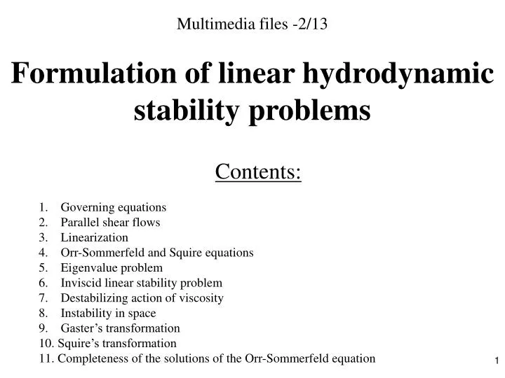
Multimedia files -2/ 13 Formulation of linear hydrodynamic stability problems. Contents : Governing equations Parallel shear flows Linearization Orr-Sommerfeld and Squire equations Eigenvalue problem Inviscid linear stability problem Destabilizing action of viscosity

E N D
Multimedia files -2/13 Formulation of linear hydrodynamic stability problems • Contents: • Governing equations • Parallel shear flows • Linearization • Orr-Sommerfeld and Squire equations • Eigenvalue problem • Inviscid linear stability problem • Destabilizing action of viscosity • Instability in space • Gaster’s transformation • Squire’s transformation • Completeness of the solutions of the Orr-Sommerfeld equation
Governing equations Euler equations NSE=momentum equations The term taking into account presence of stresses and responsible for presence for development of shear stresses (continuity equation=mass conservation) + boundary and initial conditions Streamwise (x), wall-normal (y) and spanwise (z) velocities in Cartesian coordinates r=(x,y,z) y Free stream direction j x i k z - kinematic viscosity
Reynolds number • There are many ways to derive the expression for Reynolds number and display its significance • Law of similarity: the flow about a body in simplest cases is determined by a characteristic velocity U [m/s], viscosity n [m2/s], and a characteristic size of the body L [m]. There is only one non-dimensional combination of these parameters, expressing the similarity of such flows: Re=UL/ n Any other non-dimensional parameter can be written as a function of Re. • In such a way the NS-equations can be made non-dimensional: Some of these combinations also have names, e.g., Strouhal number: St=2pfL/U, that is inverse of non-dimensional t.
U(x,y) Nonlinear disturbance equations • Let and P(r) be distributions of velocity and pressure of a known stationary solution of the Navier–Stokes equations of an incompressible fluid: • with natural boundary conditions U(S) = 0 at boundaries (walls) S. (for simplicity vector sign is removed)
Nonlinear disturbance equations, cont. Let us impose a disturbance u(r, t) and p(r,t), where r is a coordinate vector and t is time, so that the resultant motion U(r)=U(r)+u(r,t), and P(r) = P(r) + p(r, t), also satisfy the Navier–Stokes and continuity equations as well as the boundary conditions: ∂U/∂t+(U∇) U=−∇P+∇2 U/Re, (∇ U)=0. or ∂(U+u)/∂t+((U+u)∇)(U+u)=−∇P+∇2(U+u)/Re, (∇(U+u))=0. removing the parenthesis and separating the values (u,p) from (U,P) yields ∂u/∂t+(U∇)u+(u∇)U+(u∇)u=−∇p+1/R∇2u, (∇u) = 0.
Parallel shear flows NSE=momentum equations (continuity equation=mass conservation) + boundary and initial conditions The flow streamlines exhibit neither divergence nor convergence downstream: “parallel two-dimensional (2D) flow”. Assume: Local parallelity of the flow streamlines means that the streamlines diverge/converge slowly comparing with the processes of interest.
evolution equation for v Linearization and suppose that disturbances u, v, and w are small, so that the nonlinear (quadratic disturbance as u2, uv, vw,…) terms in the NS-equations can be dropped. Assume that + boundary and initial conditions equation for normal velocity:
Linearization, cont. To describe the complete three-dimensional flow field, a second equation is needed (the third one is provided by the continuity equation). This is most conveniently the equation of normal vorticity, which describes the “horizontal” flow y Free stream direction x evolution equation for + initial conditions This pair of these ordinary differential equations equations provides a complete description of the evolution of an arbitrary linear disturbance.
the Orr-Sorrmerfeld equation the Squire equation at solid walls and in free stream, with boundary conditions Orr-Sommerfeld and Squire equations The classical approach to the solution of such stability problems is the method of normal modes, consisting of a reduction of the linear initial-boundary-value problem to an eigenvalue problem. Let us suppose that the full solution can be expressed as a sum of elementary solutions (modes), which have the form Arbitrary ‘small’ complex amplitudes Then, the evolution equations for the normal velocity and normal vorticity are reduced to The OS-equation with homogeneous b.c. constitutes an eigenvalue problem for normal velocity disturbances. In the Squire equation the right-hand term depending on the normal velocity is a ‘driving’ force for the disturbances of normal vorticity.
Examples of the eigenoscillations duct solid boundary c duct solid boundary A duct with acoustic waves or electromagnetic microwave “liquid boundary” U a boundary layer with an OS mode vr solid boundary vi
OSE Solution of the Orr-Sommerfeld equation
Solution of the Squire equation imaginary part real part
k b g a Interpretation of modal results(some definitions)
Analysis and Synthesis original momentum equations for disturbances linearization solution of initial value problem reduction to eigenvalue problem (spectral analysis) expansion of any small-amplitude disturbance to the set of the modes complete set of linearly-independent modes (waves)
The instability waves related to the solutions of the Rayleigh equation are called Rayleigh waves. Note that Rayleigh equation in the final form is unchanged when a is replaced by -a. Thus, it is customary to consider a>0. Also if is an eigenfunction with c for some a then so is v* with eigenvalue c* for the same a. Thus, to each unstable mode, there exists a corresponding stable mode (* means here complex conjugation). Considering the inviscid stability problem in time for two-dimensional (direct) waves, Rayleigh proved some important general theorems. Inviscid linear stability problem
The inflection point is a point ys such that That is if the growth rate ci or wi≠0, then 2nd derivative of flow mean velocity U” profile changes sign between flow boundaries. Rayleigh’s inflection point criterion(first Rayleigh theorem) Formal multiplication of the Rayleigh equation by its complex-conjugate solution and integration by parts over y. The limits are taken [-1;+1], but this does not lead to a lack of generality. The procedure can be repeated for any other limits.
on Rayleigh’s inflection point criterion, cont.
Second Rayleigh theoremand the critical layer Rayleigh eqn. (R.E.) R.E. (for ci≠0). critical layer large velocity gradient effects of viscosity at the wall
on : Criterion of the maximum vorticity Here Us is the velocity at inflection point. Thus, only the velocity profiles with the inflection points associated with the maximum shear are unstable; i.e. the inequality U”(U-Us)<0 should be satisfied over a certain range of y. Taking into account the first Rayleigh theorem, this is equivalent to the requirement of a relative maximum of the absolute value of the vorticity at ys for the instability to occur. It follows in particular from the criterion that the Couette flow is stable in the inviscid approach. Analysis of stability of flows through the stability criteria: a stable, U’’<0; b stable, U’’>0, c stable, U’’=0, but U’’(U-Us)≥0; d probably unstable, U’’s=0 and U’(U-Us)≤0.
stable unstable Semicircle theorem Umin and Umax are minimum and maximum velocity in the flow
Behavior of u and v of 2D waveat finite Re in the critical layer Falkner-Skan basic velocity profile with backflow, bH=‒0.1 U U” a=0.06 The streamwise velocity tends to infinity in the inviscid limit like: inflection point backflow unless U''=0 in the critical layer.
As the Reyleigh inviscid instability acts at the Reynolds number Re→∞, it is clear that viscosity and, as a consequence, the viscous instability can destabilize the flow only at a finite Reynolds number. The physical mechanism of the viscous instability can be seen from the equation of energy balance: Considering two-dimensional disturbances in a parallel flow, the equation can be simplified to the form: re is a Destabilizing action of viscosity This term is zero without the shift
Examples Results of viscous computations Different asymptotic behavior at Re→∞. • That is: • The inviscid fluid may be unstable and the viscous fluid stable. The effect • of viscosity is then purely stabilizing. • The inviscid fluid may be stable and the viscous fluid unstable. In this • case viscosity would be the cause of the instability.
’ Disturbance source Disturbance source Instability in space The problem of initial conditions or stability in time. If the initial disturbance decays in time at each fixed point of space (or, at least, does not monotonically grow), the system is called stable to these disturbances. Otherwise, if the initial disturbance monotonically grows in time at a fixed point of space, the system is called absolutely unstable. In physiscs such systems are denoted sometimes as “generators”. • The problem of boundary conditions or amplification in space. If an external signal at the entrance to the system decays whilst propagating in it, it is said that the spatial attenuation (non-transmission of a signal) takes place. Otherwise, there is a spatial amplification, and the system is called convectively unstable. In physics such systems are called sometimes “amplifiers”.
evolution equation for v Difference in the evolution equations That is, we consider the development in time for the wave with given a and b.
+ Difference in the evolution equations, cont. They provide quasi-linear parabolic partial differential equations in time: Parabolic, has first order derivative in time (initial-value problem)
Development along x and z. For two-dimensional flows, the symmetry prescribe b real, so we can consider the growth only along x. s: Difference in the evolution equations, cont. Elliptic, absence of the time derivative (b.v. problem) A formulation of the later problem as the initial value problem is ill-posed, as the solution depends on the conditions at the downstream boundary and there are solutions propagating upstream. One has to regularize the problem by imposing additional constraints to the initial data. It was proposed to exclude all solutions propagating upstream. A possible physical explanation of this is a fast ‘loss’ of the effect of the downstream boundary conditions in the bulk of the boundary layer or channel flow due to a quick decay of the upstream propagating disturbances. We will show this by considering the structure of the spectrum of the Orr-Sommerfeld and Squire equations.
Eigenvalue problem OS SQ Note that negative ai correspond to unstable disturbances, because of the factor: ei(ax+by-wt)=e-aiei(arx+by-wt). The OS-equation constitutes the 4th order polynomial (sometimes called “nonlinear”) eigenvalue problem in a.
Gaster’s transformation, cont. The prove is centered in considering the total differential of the general form of the disturbance relation about a neutral disturbance in complex plane. Using it we obtain: values at thу neutral curve relates small changes in a to small changes in w through the group velocity For strongly unstable flows, the transformation is not accurate, as it is based on a linear expansion about a neutral value.
Inviscid instability in space • The Rayleigh theorems is impossible to prove for complex a. • However, the results for neutral disturbances are equally applicable for both cases. • For non-neutral cases (slightly stable or unstable) the Gaster’s transformation is applicable.
Squire’s transformation It is clear that both equations are equivalent, if put
Completeness of the solutions of the Orr-Sommerfeld equation For the OS and Squire equations a proof is required for the completeness of the solutions.
Structure of the solutionsof the Orr-Sommerfeld equation(pressure waves) vr vi
Structure of the solutionsof the Orr-Sommerfeld equation(vorticity waves) upstream of the source downstream vi vr
Structure of the solutionsof the Orr-Sommerfeld equation(discrete waves)
Further reading • Betchov R. and Criminale W. O. (1967) Stability of parallel flows, NY: Academic. • Drazin P. G. and Reid W. H. (1981) Hydrodynamic Stability, Cambridge University Press • Gaster M. (1962) A note on the relation between temporally-increasing and spatially-increasing disturbances in hydrodynamic stability, J. Fluid Mech., Vol. 14, pp. 222‒224. • Schmid P.J., Henningson D.S. (2000) Stability and transition in shear flows, Springer, p. 1‒60.