Download
1 / 30
310 likes | 522 Views
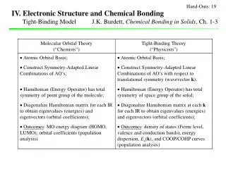
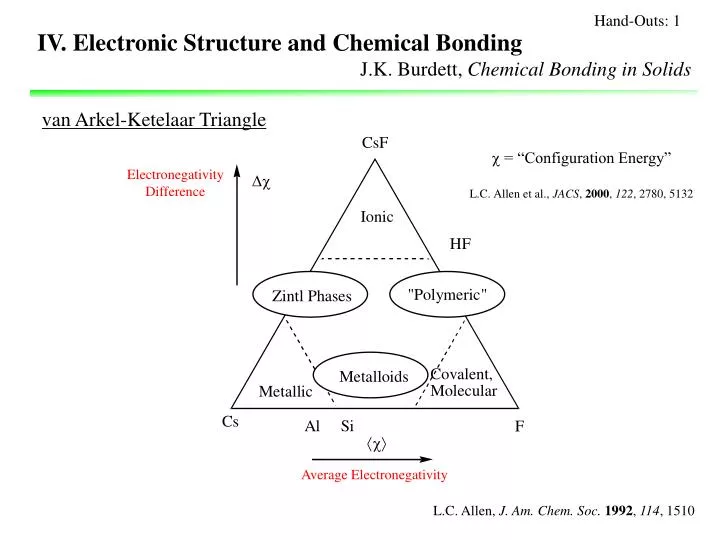
Hand-Outs: 1. IV. Electronic Structure and Chemical Bonding J.K. Burdett, Chemical Bonding in Solids. van Arkel-Ketelaar Triangle. = “Configuration Energy” L.C. Allen et al., JACS , 2000 , 122 , 2780, 5132. Electronegativity Difference. Average Electronegativity.

E N D
Hand-Outs: 1 IV. Electronic Structure and Chemical Bonding J.K. Burdett, Chemical Bonding in Solids van Arkel-Ketelaar Triangle • = “Configuration Energy” L.C. Allen et al., JACS, 2000, 122, 2780, 5132 Electronegativity Difference Average Electronegativity L.C. Allen, J. Am. Chem. Soc. 1992, 114, 1510
IV. Electronic Structure and Chemical Bonding J.K. Burdett, Chemical Bonding in Solids • Schrödinger’s Equation: {n} = E{n}{n} • “A solid is a molecule with an infinite number (ca. 1023)of atoms.” • Molecular Solids: on molecular entities (as in gas phase); packing effects? • Extended Solids: how to make the problem tractable? • (a) Amorphous (glasses): silicates, phosphates – molecular fragments, tie • off ends with simple atoms, e.g., “H”; • (b) Quasiperiodic: fragments based on building units, tie off ends with • simple atoms, e.g., “H”; • (c) Crystalline: unit cells (translational symmetry) – elegant simplification!
IV. Electronic Structure and Chemical Bonding J.K. Burdett, Chemical Bonding in Solids Electronic Structure of Si: Fermi Level Electronic Band Structure Electronic Density of States What can we learn from this information?
Hand-Outs: 5 IV. Electronic Structure and Chemical Bonding Bloch’s Theorem The wavefunctions for electrons, phonons (= lattice vibrations) subjected to periodic potential, i.e., U(r + t) = U(r), take the form nk(r) = eikr un(r) where un(r) has the full periodicity of the lattice, i.e., un(r + t) = un(r). Note that nk(r + t) = eikt nk(r) Therefore, for a determination of electronic states or vibrational modes in crystals, we only need to treat the contents of the unit cell (primitive cell)!
Hand-Outs: 6 IV. Electronic Structure and Chemical Bonding Crystalline Wavefunctions: Rotational Symmetry nk(r): n = quantum numbers (IRs) for rotational symmetry; k = quantum numbers (IRs) for translational symmetry (confined within first Brillouin zone) Example: Square lattice (C4v symmetry) v d v d {E, C4, C42, C43, 2v, 2d}
Hand-Outs: 6 IV. Electronic Structure and Chemical Bonding Crystalline Wavefunctions: Rotational Symmetry nk(r): n = quantum numbers (IRs) for rotational symmetry; k = quantum numbers (IRs) for translational symmetry (confined within first Brillouin zone) Example: Square lattice (C4v symmetry) (2/a, 0) v d FBZ v (0, 2/a) (0,0) (0, 2/a) d {E, C4, C42, C43, 2v, 2d} The rotational symmetry of reciprocal space is the same as real space. (2/a, 0) Reciprocal Space
Hand-Outs: 6 IV. Electronic Structure and Chemical Bonding Crystalline Wavefunctions: Rotational Symmetry nk(r): n = quantum numbers (IRs) for rotational symmetry; k = quantum numbers (IRs) for translational symmetry (confined within first Brillouin zone) Example: Square lattice (C4v symmetry) Reciprocal Space {E, C4, C42, C43, 2v, 2d} Star of k 1 wavevector FBZ (0, 0) Group of the Wavevector k = (0, 0): “C4v” nk=0 are basis functions for “C4v”
Hand-Outs: 6 IV. Electronic Structure and Chemical Bonding Crystalline Wavefunctions: Rotational Symmetry nk(r): n = quantum numbers (IRs) for rotational symmetry; k = quantum numbers (IRs) for translational symmetry (confined within first Brillouin zone) Example: Square lattice (C4v symmetry) Reciprocal Space {E, C4, C42, C43, 2v, 2d} Star of k 4 wavevectors FBZ (0, ky) Group of the Wavevector k = (0, ky): “Cs” nk= are basis functions for “Cs”
Hand-Outs: 6 IV. Electronic Structure and Chemical Bonding Crystalline Wavefunctions: Rotational Symmetry nk(r): n = quantum numbers (IRs) for rotational symmetry; k = quantum numbers (IRs) for translational symmetry (confined within first Brillouin zone) Example: Square lattice (C4v symmetry) Reciprocal Space {E, C4, C42, C43, 2v, 2d} Star of k 2 wavevectors FBZ X (0, /a) Group of the Wavevector k = X (0, /a): “C2v” nk=X are basis functions for “C2v”
Hand-Outs: 6 IV. Electronic Structure and Chemical Bonding Crystalline Wavefunctions: Rotational Symmetry nk(r): n = quantum numbers (IRs) for rotational symmetry; k = quantum numbers (IRs) for translational symmetry (confined within first Brillouin zone) Example: Square lattice (C4v symmetry) Reciprocal Space {E, C4, C42, C43, 2v, 2d} Star of k 4 wavevectors FBZ Z (kx, /a) Group of the Wavevector k = Z (kx, /a): “Cs” nk=Z are basis functions for “Cs”
Hand-Outs: 6 IV. Electronic Structure and Chemical Bonding Crystalline Wavefunctions: Rotational Symmetry nk(r): n = quantum numbers (IRs) for rotational symmetry; k = quantum numbers (IRs) for translational symmetry (confined within first Brillouin zone) Example: Square lattice (C4v symmetry) Reciprocal Space {E, C4, C42, C43, 2v, 2d} Star of k 1 wavevector FBZ M (/a, /a) Group of the Wavevector k = M (/a, /a): “C4v” nk=M are basis functions for “C4v”
Hand-Outs: 6 IV. Electronic Structure and Chemical Bonding Crystalline Wavefunctions: Rotational Symmetry nk(r): n = quantum numbers (IRs) for rotational symmetry; k = quantum numbers (IRs) for translational symmetry (confined within first Brillouin zone) Example: Square lattice (C4v symmetry) Reciprocal Space {E, C4, C42, C43, 2v, 2d} Star of k 4 wavevectors FBZ (k, k) Group of the Wavevector k = (k, k): “Cs” nk= are basis functions for “Cs”
Hand-Outs: 6 IV. Electronic Structure and Chemical Bonding Crystalline Wavefunctions: Rotational Symmetry nk(r): n = quantum numbers (IRs) for rotational symmetry; k = quantum numbers (IRs) for translational symmetry (confined within first Brillouin zone) Example: Square lattice (C4v symmetry) Reciprocal Space {E, C4, C42, C43, 2v, 2d} Star of k 8 wavevectors FBZ General Point Order of the Point Group of the Space Group Order of the Group of the Wavevector # vectors in the star of k = Group of the Wavevector k = (kx, ky): “C1” nk= are basis functions for “C1”
Hand-Outs: 6 IV. Electronic Structure and Chemical Bonding Crystalline Wavefunctions: Rotational Symmetry nk(r): n = quantum numbers (IRs) for rotational symmetry; k = quantum numbers (IRs) for translational symmetry (confined within first Brillouin zone) Example: Square lattice (C4v symmetry) Reciprocal Space v d FBZ v X d {E, C4, C42, C43, 2v, 2d} M “Irreducible Wedge” (1/8 area of First Brillouin Zone) (Minimum volume (area) of Brillouin Zone containing energetic information)
Hand-Outs: 7-8 IV. Electronic Structure and Chemical Bonding Brillouin Zones Melvin Lax, Symmetry Principles in Solid State and Molecular Physics Irreducible Wedges (Laue Classes)
Fermi Level Hand-Outs: 9 IV. Electronic Structure and Chemical Bonding J.K. Burdett, Chemical Bonding in Solids Electronic Structure of Si Conduction Band 3p (“t”) Valence Band Si-Si Bonding 3s (“a”) “D3d” “Oh”
Fermi Level Hand-Outs: 9 IV. Electronic Structure and Chemical Bonding J.K. Burdett, Chemical Bonding in Solids Electronic Structure of Si How are these diagrams determined?
Hand-Outs: 10 IV. Electronic Structure and Chemical Bonding Methods R. Dronskowski, Computational Chemistry of Solid State Materials n = (T + U) n = Enn = [(e + ne) + ee] n = [(e + ne) + (ee,Coul + ee,XC)] n Empirical / Semi-empirical: (use energy parameters based on experiment) “One-electron” methods: Hückel, Extended Hückel (EHT) many approximations (explicitly ignore ee); fast; useful (successful) when symmetry effects are important First Principles: (calculate all terms based on physical models) Hartree-Fock: good for insulators & semiconductors; poor for metals (“Fermi liquid”) Density Functional Theory (DFT): based on electron density; suited for ground-state properties (structures, charge density) – band gaps underestimated for semicond. Local Density Approx. (LDA): ee,XC modeled by free electron gas Local Spin Density Approx. (LSDA): same as LDA but different for different spins Correlation: LDA + U; rare-earth ions (localized 4f electrons), transition metals in salts (metal oxides).
Hand-Outs: 10 IV. Electronic Structure and Chemical Bonding Models R. Dronskowski, Computational Chemistry of Solid State Materials n = (T + U) n = Enn = [(e + ne) + ee] n = [(e + ne) + (ee,Coul + ee,XC)] n Free Electron Method (e and ee only) Nearly Free Electron (ne included) Pseudopotential (include core-valence effects in ne) Cellular (Augmentation) Approach Linear Methods Atomic Sphere Approximation (ASA) Tight Binding (“Molecular Orbital”) L.C.A.O. “Strong” atomic potential
Hand-Outs: 10 IV. Electronic Structure and Chemical Bonding Models R. Dronskowski, Computational Chemistry of Solid State Materials n = (T + U) n = Enn = [(e + ne) + ee] n = [(e + ne) + (ee,Coul + ee,XC)] n Free Electron Method (e and ee only) Nearly Free Electron (ne included) Pseudopotential Cellular (Augmentation) Approach Linear Methods Atomic Sphere Approximation (ASA) Tight Binding (“Molecular Orbital”) L.C.A.O. “Strong” atomic potential Programs EHMACC (EHT) YAeHMOP(EHT) CRYSTAL (Hartree-Fock) TB-LMTO (Cellular) VASP(Pseudopotential) FLMTO(Cellular) WIEN2k(Cellular)
Hand-Outs: 11 IV. Electronic Structure and Chemical Bonding Models n = (T + U) n = Enn = [(e + ne) + ee] n = [(e + ne) + (ee,Coul + ee,XC)] n Free Electron Method (e and ee only) Nearly Free Electron (ne included) Pseudopotential (include core-valence effects in ne) Cellular (Augmentation) Approach Linear Methods Atomic Sphere Approximation (ASA) Tight Binding (“Molecular Orbital”) L.C.A.O. “Strong” atomic potential
M M M M M M M M M M M M M M M M M Hand-Outs: 11 IV. Electronic Structure and Chemical Bonding Cellular Approach Divide a structure into Wigner-Seitz cells; nk must be continuous at boundaries BUT, unusual (polyhedral) shapes of WS cells make this solution challenging, so…
M M M M M M M M M M M M M M M M M M M M M M M M M M M M M M M M M M Hand-Outs: 11 IV. Electronic Structure and Chemical Bonding Cellular Approach Divide a structure into Wigner-Seitz cells; nk must be continuous at boundaries “Atomic-like” (Spherical) Potential “Free Electron-like” (Constant) Potential BUT, unusual (polyhedral) shapes of WS cells make this solution challenging, so… RWS = radius of sphere
M M M M M M M M M M M M M M M M M M M M M M M M M M M M M M M M M M Hand-Outs: 11 IV. Electronic Structure and Chemical Bonding Cellular Approach • Simplifications (Approximation) • Atomic-Sphere-Approximation (ASA) • Linear method (fast)
Hand-Outs: 12 IV. Electronic Structure and Chemical Bonding Free Electron Model (“Jellium,” “Homogeneous Electron Gas”) Important Parameter: Density of Free (Conduction) Electrons, (r) Electronic Energy = Kinetic Energy (p2/2m); Potential Energy is constant (= 0) Schrödinger’s Equation: Wavefunctions (Plane waves) Quantum Numbers (Wavevectors k): Energies (Kinetic Energy) (Electron momentum)
Hand-Outs: 12 IV. Electronic Structure and Chemical Bonding Free Electron Model (“Jellium,” “Homogeneous Electron Gas”) Important Parameter: Density of Free (Conduction) Electrons, (r) Electronic Energy = Kinetic Energy (p2/2m); Potential Energy is constant (= 0) Schrödinger’s Equation: Wavefunctions (Plane waves) Quantum Numbers (Wavevectors k): Energies (Kinetic Energy) (Electron momentum) As V (L) increases, the density of allowed states, k, increases. Volume / k-point = Therefore, # k-points per volume is
Hand-Outs: 12 IV. Electronic Structure and Chemical Bonding Free Electron Model Unoccupied States Fermi Level Occupied States Fermi Wavevector 0
Hand-Outs: 12 IV. Electronic Structure and Chemical Bonding Free Electron Model Wavefunction (“Orbital”) = k (Each holds at most 2 electrons) Unoccupied States Fermi Level Occupied States kz Fermi Sphere Radius = kF ky Fermi Wavevector kx 0
Hand-Outs: 12 IV. Electronic Structure and Chemical Bonding Free Electron Model Wavefunction (“Orbital”) = k (Each holds at most 2 electrons) Unoccupied States Fermi Level Occupied States kz Fermi Sphere Radius = kF ky Fermi Wavevector kx 0
Hand-Outs: 12 IV. Electronic Structure and Chemical Bonding Free Electron Model (Terms; Units) Radius of Sphere containing 1 electron = rs (Bohr radius = 0.529 Å) Fermi Wavevector = kF Fermi Energy = Energy of Highest Occupied “Orbital” (Rydberg = 13.6 eV) Electron Density =