Download
1 / 68
680 likes | 682 Views
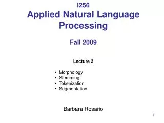
I256: Applied Natural Language Processing. Marti Hearst October 18, 2006 (Many slides originally by Barbara Rosario, modified here). Today. Algorithms for Classification Binary classification Perceptron Winnow Support Vector Machines (SVM) Kernel Methods Multi-Class classification

E N D
I256: Applied Natural Language Processing Marti Hearst October 18, 2006 (Many slides originally by Barbara Rosario, modified here)
Today • Algorithms for Classification • Binary classification • Perceptron • Winnow • Support Vector Machines (SVM) • Kernel Methods • Multi-Class classification • Decision Trees • Naïve Bayes • K nearest neighbor
Binary Classification: examples • Spam filtering (spam, not spam) • Customer service message classification (urgent vs. not urgent) • Information retrieval (relevant, not relevant) • Sentiment classification (positive, negative) • Sometime it can be convenient to treat a multi-way problem like a binary one: one class versus all the others, for all classes
Binary Classification • Given: some data items that belong to a positive (+1 ) or a negative (-1 ) class • Task: Train the classifier and predict the class for a new data item • Geometrically: find a separator
Linear versus Non Linear algorithms • Linearly separable data: if all the data points can be correctly classified by a linear (hyperplanar) decision boundary
Class1 Linear Decision boundary Class2 Linearly separable data
Class1 Class2 Non linearly separable data
Class1 Class2 Non linearly separable data Non LinearClassifier
Linear versus Non Linear algorithms • Linear or Non linear separable data? • We can find out only empirically • Linear algorithms (algorithms that find a linear decision boundary) • When we think the data is linearly separable • Advantages • Simpler, less parameters • Disadvantages • High dimensional data (like for NLT) is usually not linearly separable • Examples: Perceptron, Winnow, SVM • Note: we can use linear algorithms also for non linear problems (see Kernel methods)
Linear versus Non Linear algorithms • Non Linear • When the data is non linearly separable • Advantages • More accurate • Disadvantages • More complicated, more parameters • Example: Kernel methods • Note: the distinction between linear and non linear applies also for multi-class classification (we’ll see this later)
Simple linear algorithms • Perceptron and Winnow algorithm • Linear • Binary classification • Online (process data sequentially, one data point at the time) • Mistake driven • Simple single layer Neural Networks
Linear binary classification • Data:{(xi,yi)}i=1...n • x in Rd (x is a vector in d-dimensional space) feature vector • y in {-1,+1} label (class, category) • Question: • Design a linear decision boundary: wx + b (equation of hyperplane) such that the classification rule associated with it has minimal probability of error • classification rule: • y = sign(wx + b) which means: • if wx + b > 0 then y = +1 • if wx + b < 0 then y = -1 From Gert Lanckriet, Statistical Learning Theory Tutorial
Linear binary classification • Finda good hyperplane (w,b) in Rd+1 that correctly classifies data points as much as possible • In online fashion: one data point at the time, update weights as necessary wx + b = 0 Classification Rule: y = sign(wx + b) From Gert Lanckriet, Statistical Learning Theory Tutorial
wk+1 Wk+1 x + b = 0 Perceptron algorithm • Initialize:w1 = 0 • Updating ruleFor each data point x • If class(x) != decision(x,w) • then wk+1 wk + yixi k k + 1 • else wk+1 wk • Function decision(x, w) • If wx + b > 0 return +1 • Else return -1 wk +1 0 -1 wk x + b = 0 From Gert Lanckriet, Statistical Learning Theory Tutorial
Perceptron algorithm • Online: can adjust to changing target, over time • Advantages • Simple and computationally efficient • Guaranteed to learn a linearly separable problem (convergence, global optimum) • Limitations • Only linear separations • Only converges for linearly separable data • Not really “efficient with many features” From Gert Lanckriet, Statistical Learning Theory Tutorial
Winnow algorithm • Another online algorithm for learning perceptron weights: f(x) = sign(wx + b) • Linear, binary classification • Update-rule: again error-driven, but multiplicative (instead of additive) From Gert Lanckriet, Statistical Learning Theory Tutorial
wk+1 Wk+1 x + b = 0 Winnow algorithm • Initialize:w1 = 0 • Updating ruleFor each data point x • If class(x) != decision(x,w) • then wk+1 wk + yixi Perceptron wk+1 wk *exp(yixi) Winnow k k + 1 • else wk+1 wk • Function decision(x, w) • If wx + b > 0 return +1 • Else return -1 wk +1 0 -1 wk x + b= 0 From Gert Lanckriet, Statistical Learning Theory Tutorial
Perceptron vs. Winnow • Assume • N available features • only K relevant items, with K<<N • Perceptron: number of mistakes: O( K N) • Winnow: number of mistakes: O(K log N) Winnow is more robust to high-dimensional feature spaces From Gert Lanckriet, Statistical Learning Theory Tutorial
Perceptron Online: can adjust to changing target, over time Advantages Simple and computationally efficient Guaranteed to learn a linearly separable problem Limitations only linear separations only converges for linearly separable data not really “efficient with many features” Winnow Online: can adjust to changing target, over time Advantages Simple and computationally efficient Guaranteed to learn a linearly separable problem Suitable for problems with many irrelevant attributes Limitations only linear separations only converges for linearly separable data not really “efficient with many features” Used in NLP Perceptron vs. Winnow From Gert Lanckriet, Statistical Learning Theory Tutorial
Large margin classifier • Another family of linear algorithms • Intuition (Vapnik, 1965) • If the classes are linearly separable: • Separate the data • Place hyper-plane “far” from the data: large margin • Statistical results guarantee good generalization BAD From Gert Lanckriet, Statistical Learning Theory Tutorial
Large margin classifier • Intuition (Vapnik, 1965) if linearly separable: • Separate the data • Place hyperplane “far” from the data: large margin • Statistical results guarantee good generalization GOOD Maximal Margin Classifier From Gert Lanckriet, Statistical Learning Theory Tutorial
Large margin classifier If not linearly separable • Allow some errors • Still, try to place hyperplane “far” from each class From Gert Lanckriet, Statistical Learning Theory Tutorial
Large Margin Classifiers • Advantages • Theoretically better (better error bounds) • Limitations • Computationally more expensive, large quadratic programming
wTxa + b = 1 M wTxb + b = -1 wT x + b = 0 Support vectors Support Vector Machine (SVM) • Large Margin Classifier • Linearly separable case • Goal: find the hyperplane that maximizes the margin From Gert Lanckriet, Statistical Learning Theory Tutorial
Support Vector Machine (SVM) • Text classification • Hand-writing recognition • Computational biology (e.g., micro-array data) • Face detection • Face expression recognition • Time series prediction From Gert Lanckriet, Statistical Learning Theory Tutorial
Non Linear problem • Kernel methods • A family of non-linear algorithms • Transform the non linear problem in a linear one (in a different feature space) • Use linear algorithms to solve the linear problem in the new space From Gert Lanckriet, Statistical Learning Theory Tutorial
Main intuition of Kernel methods • (Copy here from black board)
wT(x)+b=0 (X)=[x2 z2 xz] f(x) = sign(w1x2+w2z2+w3xz +b) Basic principle kernel methods : Rd RD (D >> d) X=[x z] From Gert Lanckriet, Statistical Learning Theory Tutorial
Basic principle kernel methods • Linear separability: more likely in high dimensions • Mapping: maps input into high-dimensional feature space • Classifier: construct linear classifier in high-dimensional feature space • Motivation: appropriate choice of leads to linear separability • We can do this efficiently! From Gert Lanckriet, Statistical Learning Theory Tutorial
Basic principle kernel methods • We can use the linear algorithms seen before (Perceptron, SVM) for classification in the higher dimensional space
Multi-class classification • Given: some data items that belong to one of M possible classes • Task: Train the classifier and predict the class for a new data item • Geometrically: harder problem, no more simple geometry
Multi-class classification: Examples • Author identification • Language identification • Text categorization (topics)
(Some) Algorithms for Multi-class classification • Linear • Parallel class separators: Decision Trees • Non parallel class separators: Naïve Bayes • Non Linear • K-nearest neighbors
Decision Trees • Decision tree is a classifier in the form of a tree structure, where each node is either: • Leaf node - indicates the value of the target attribute (class) of examples, or • Decision node - specifies some test to be carried out on a single attribute-value, with one branch and sub-tree for each possible outcome of the test. • A decision tree can be used to classify an example by starting at the root of the tree and moving through it until a leaf node, which provides the classification of the instance. http://dms.irb.hr/tutorial/tut_dtrees.php
Day Outlook Temp. Humidity Wind Play Tennis D1 Sunny Hot High Weak No D2 Sunny Hot High Strong No D3 Overcast Hot High Weak Yes D4 Rain Mild High Weak Yes D5 Rain Cool Normal Weak Yes D6 Rain Cool Normal Strong No D7 Overcast Cool Normal Weak Yes D8 Sunny Mild High Weak No D9 Sunny Cold Normal Weak Yes D10 Rain Mild Normal Strong Yes D11 Sunny Mild Normal Strong Yes D12 Overcast Mild High Strong Yes D13 Overcast Hot Normal Weak Yes D14 Rain Mild High Strong No Training Examples Goal: learn when we can play Tennis and when we cannot
Decision Tree for PlayTennis Outlook Sunny Overcast Rain Humidity Yes Wind High Normal Strong Weak No Yes No Yes www.math.tau.ac.il/~nin/ Courses/ML04/DecisionTreesCLS.pp
Each internal node tests an attribute Each branch corresponds to an attribute value node Each leaf node assigns a classification Decision Tree for PlayTennis Outlook Sunny Overcast Rain Humidity High Normal No Yes www.math.tau.ac.il/~nin/ Courses/ML04/DecisionTreesCLS.pp
No Outlook Sunny Overcast Rain Humidity Yes Wind High Normal Strong Weak No Yes No Yes Decision Tree for PlayTennis Outlook Temperature Humidity Wind PlayTennis Sunny Hot High Weak ? www.math.tau.ac.il/~nin/ Courses/ML04/DecisionTreesCLS.pp
Decision Tree for Reuter classification Foundations of Statistical Natural Language Processing, Manning and Schuetze
Decision Tree for Reuter classification Foundations of Statistical Natural Language Processing, Manning and Schuetze
Building Decision Trees • Given training data, how do we construct them? • The central focus of the decision tree growing algorithm is selecting which attribute to test at each node in the tree. The goal is to select the attribute that is most useful for classifying examples. • Top-down, greedy search through the space of possible decision trees. • That is, it picks the best attribute and never looks back to reconsider earlier choices.
Building Decision Trees • Splitting criterion • Finding the features and the values to split on • for example, why test first “cts” and not “vs”? • Why test on “cts < 2” and not “cts < 5” ? • Split that gives us the maximum information gain (or the maximum reduction of uncertainty) • Stopping criterion • When all the elements at one node have the same class, no need to split further • In practice, one first builds a large tree and then one prunes it back (to avoid overfitting) • SeeFoundations of Statistical Natural Language Processing, Manning and Schuetze for a good introduction
Decision Trees: Strengths • Decision trees are able to generate understandable rules. • Decision trees perform classification without requiring much computation. • Decision trees are able to handle both continuous and categorical variables. • Decision trees provide a clear indication of which features are most important for prediction or classification. http://dms.irb.hr/tutorial/tut_dtrees.php
Decision Trees: weaknesses • Decision trees are prone to errors in classification problems with many classes and relatively small number of training examples. • Decision tree can be computationally expensive to train. • Need to compare all possible splits • Pruning is also expensive • Most decision-tree algorithms only examine a single field at a time. This leads to rectangular classification boxes that may not correspond well with the actual distribution of records in the decision space. http://dms.irb.hr/tutorial/tut_dtrees.php