Download
1 / 17
230 likes | 786 Views
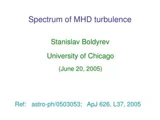
Spectrum of MHD turbulence. Stanislav Boldyrev. University of Chicago. (June 20, 2005). Ref: astro-ph/0503053; ApJ 626, L37, 2005. Introduction: Kolmogorov turbulence. Random flow of incompressible fluid. Reynolds number:. v. L. Re=Lv/ η >>1. η -viscosity.

E N D
Spectrum of MHD turbulence Stanislav Boldyrev University of Chicago (June 20, 2005) Ref: astro-ph/0503053; ApJ 626, L37, 2005
Introduction: Kolmogorov turbulence Random flow of incompressible fluid Reynolds number: v L Re=Lv/η>>1 η-viscosity If there is no intermittency, then: and Kolmogorov spectrum [Kolmogorov 1941]
Kolmogorov energy cascade local energy flux Energy of an eddy of size is ; it is transferred to a smaller-size eddy during time: - “eddy turn-over” time. , is constant for the The energy flux, Kolmogorov spectrum!
MHD turbulence No exact Kolmogorov relation. Phenomenology: is conserved, and cascades toward small scales. Energy No, since dimensional arguments do not work! ? • Is energy transfer time Non-dimensional parameter can enter the answer. • Need to investigate interaction of “eddies” in detail! This is also the main problem in the theory of weak (wave) turbulence. (waves is plasmas, water, solid states, liquid helium, etc…) [Kadomtsev, Zakharov, ... 1960’s]
w z z w Iroshnikov-Kraichnan spectrum After interaction, shape of each packet changes, but energy does not.
Iroshnikov-Kraichnan spectrum during one collision: number of collisions required to deform packet considerably: λ λ Constant energy flux: [Iroshnikov (1963); Kraichnan (1965)]
L>> λ B ┴ Goldreich-Sridhar theory Anisotropy of “eddies” B λ L Shear Alfvén waves dominate the cascade: Critical Balance [Goldreich & Sridhar (1995)]
Spectrum of MHD Turbulence in Numerics [Müller & Biskamp, PRL 84 (2000) 475]
Goldreich-Sridhar Spectrum in Numerics Cho & Vishniac, ApJ, 539, 273, 2000 Cho, Lazarian & Vishniac, ApJ, 564, 291, 2002
Strong Magnetic Filed, Numerics Contradictions with Goldreich-Sridhar model Iroshnikov-Kraichnan scaling [Maron & Goldreich, ApJ 554, 1175, 2001]
B-parallel scaling B-perp scaling Strong Magnetic Filed, Numerics Contradictions with Goldreich-Sridhar model Scaling of field-parallel and field-perpendicular structure functions for different large-scale magnetic fields. [Müller, Biskamp, Grappin PRE, 67, 066302, 2003] Weak field, B→0: Goldreich-Sridhar (Kolmogorov) scaling 2 Strong field, B>>ρV : Iroshnikov-Kraichnan scaling
1 1 2 2 For perturbation cannot propagate along the B-line faster than V , therefore, correlation length along the line is A This balances terms and in the MHD equations, as in the Goldreich-Sridhar picture, however, the geometric meaning is different. New Model for MHD Turbulence Analytic Introduction [S.B., ApJ, 626, L37,2005] Depletion of nonlinear interaction: Nonlinear interaction is depleted Interaction time is increased
Goldreich-Sridhar scaling corresponds to α=0: “Iroshnikov-Kraichnan” scaling is reproduced for α=1: New Model for MHD Turbulence Analytic Introduction [S.B., ApJ, 626, L37,2005] Nonlinear interaction is depleted Interaction time is increased Constant energy flux, Explains numerically observed scalings for strong B-field ! [Maron & Goldreich, ApJ 554, 1175, 2001] [Müller, Biskamp, Grappin PRE, 67, 066302, 2003]
S.B. (2005) “eddy”: Goldreich-Sridhar 1995 “eddy”: line displacement: line displacement: turns into filament turns into current sheet agrees with numerics! New Model for MHD Turbulence Geometric Meaning As the scale decreases, λ→0,
New Model for MHD Turbulence Depletion of nonlinearity S.B. (2005) “eddy”: line displacement: In our “eddy”, w and z are aligned within small angle . One can check that: θ λ θ In our theory, this angle is: Remarkably, we reproduced the reduction factor in the original formula: The theory is self-consistent.
1.Weak large-scale field: [Goldreich & Sridhar’ 95] dissipative structures: filaments -5/3 energy spectrum: E(K)~K ┴ 2.Strong large-scale field: scale-dependent dynamic alignment dissipative structures: current sheets energy spectrum: E(K)~K -3/2 ┴ 3. The spectrum of MHD turbulence may be non-universal. Alternatively, it may always be E~K ,but in case1,resolution of numerical simulations is not large enough to observe it. -3/2 ┴ Summary and Discussions
Conclusions • Theory is proposed that explains contradiction between • Goldreich-Sridhar theory and numerical findings. • In contrast with GS theory, we predict that turbulent eddies • are three-dimensionally anisotropic, and that dissipative • structures are current sheets. • For strong large-scale magnetic field, the energy spectrum • is E~K . It is quite possible that spectrum is always E~K , • but for weak large-scale field, the resolution of numerical • simulations is not large enough to observe it. -3/2 -3/2 ┴ ┴