Download
1 / 33
330 likes | 419 Views
3-Dim Problems. 3-D Problems. Separation of Variables Y (r qf ) = R(r) Q ( q ) F ( f ) F ( f ) solution Q ( q ) solution R(r) equation Effective Potentials. Separation of Variables. Coordinates & Normalization. r. Note derivatives are cleanly separated. {a}. {b}. {c}. {d}. {d}.

E N D
3-D Problems • Separation of Variables • Y(rqf) = R(r) Q(q) F(f) • F(f) solution • Q(q) solution • R(r) equation • Effective Potentials
{a} {b} {c} {d}
{d} {e} LHS = const = RHS m2 {f}
Azimuthal Behavior …, -2, -1, 0, 1, 2, … Note: 1) EVP 2) Since no V involved only have to do this once forevermore
Other Piece {f} {g} {h} {i} {j}
{j} LHS = const = RHS {k} {l}
Other Angular Piece (co-lattitude) {l} Note: 1) EVP 2) Since no V involved only have to do this once forevermore Solns depend on choice of both l and m Associated Legendre Polynomials defer solving til later when we have nicer techniques
Summarizing the Angular Parts So Far Since the angular basis functions are the same regardless of the potential chosen. John Day @ http://www.cloudman.com/gallery1/gallery1_2.html Define the “spherical harmonics” http://asd-www.larc.nasa.gov/cgi-bin/SCOOL_Clouds/Cumulus/list.cgi
http://asd-www.larc.nasa.gov/cgi-bin/SCOOL_Clouds/Cumulus/list.cgihttp://asd-www.larc.nasa.gov/cgi-bin/SCOOL_Clouds/Cumulus/list.cgi
http://www2.physics.umd.edu/~gcchang/courses/phys402/common/notebooks.htmlhttp://www2.physics.umd.edu/~gcchang/courses/phys402/common/notebooks.html
Radial Piece {k} effective potential Note: 1) EVP 2) This has to be solved for every different choice of V(r) 3) Will determine the allowed Etot ‘s
http://asd-www.larc.nasa.gov/cgi-bin/SCOOL_Clouds/Cumulus/list.cgihttp://asd-www.larc.nasa.gov/cgi-bin/SCOOL_Clouds/Cumulus/list.cgi Summary So Far
Effective Potential Depends on the forces involved Atomic motion? Nuclear motion? … Centripetal Term
Bare Coulomb Potential He Li Be B C * * * H-atom positronium atom
Effective Potential: H atom Free States Etot > 0 l = 0 Etot Bound States Etot < 0 Atomic Potential Example Vcoul := -14.42/r 1 := 1 Vorbital := 3.818 * 1* (1+1) /r^2 Veff := Vcoul + Vorbital Plot[ {Vcoul, Vorbital, Veff}, {r, 0.3, 8}, PlotStyle ~ {{RGBColor[0, 0,1]}, {RGBColor[0, 1,0]}, {RGBColor[l, 0,0]}}, AxesLabel ~ {"r (A)", "Energy (eV)"}]
Electron Clouds – dot plots http://www.uark.edu/misc/julio/orbitals/ Scatter plots of hydrogen-atom wavefunctions This is a tentative project. The figures that you can link to from this page are made by choosing 2000 points at random, with a probability given by one of the hydrogen atom's wavefunctions. The resulting plots give an idea of the "shape" of the atomic wavefunctions. You can rotate them by clicking and dragging with the mouse; you can also magnify the figure by clicking and dragging vertically while holding down the "shift" key. The points were generated in Mathematica and the interactive figures were generated using LiveGraphics3D. LiveGraphics3D is an applet (not written by me); for it to work, you need to have java enabled in your browser.
Effective Potential: H atom l = 1 Bound States Etot < 0 Atomic Potential Example Vcoul := -14.42/r 1 := 1 Vorbital := 3.818 * 1* (1+1) /r^2 Veff := Vcoul + Vorbital Plot[ {Vcoul, Vorbital, Veff}, {r, 0.3, 8}, PlotStyle ~ {{RGBColor[0, 0,1]}, {RGBColor[0, 1,0]}, {RGBColor[l, 0,0]}}, AxesLabel ~ {"r (A)", "Energy (eV)"}]
Bound States Etot < 0 l = 1 l = 2
Effective Potential: Nuclear Examples l = 1 Vo := -50 R := 4 a:= 0.67 VNcentral = Vo / (l+Exp[(r-R)/a]) VNorbital := (197*197/2/940) * 1* (1+1) / r^2 VNeff : = VNcentral + VNorbital Plot[ {VNcentral, VNorbital, VNeff}, {r, 0.3, 10.0}, PlotStyle ~ {{RGBColor[0, 0,1]}, {RGBColor[0, 1,0]}, {RGBColor[l, 0,0]}}, AxesLabel ~ {"r (fm)", "Energy (MeV)"}]
Bound States Etot ~< 0 l = 0 l = 1 l = 2
Zoom in free particles Etot > Vtop quasi-free Vtop > Etot > 0 quasi-bound l = 2 a small positive barrier appears “Centripetal barrier”
Zoom in Application to Radioactive Alpha Decay Etot 238U = ( 234Th + a ) 234Th + a
Zoom in Neutron-Induced Reactions Etot Neutrons with l = 0 have NO centripetal barrier and are most efficient for creating nuclear reactions