TKO: Top K Outlier Detector Use D 2 NN =rank 2 S x for TopKOutlier -slider .

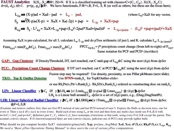
FAUST Analytics X(X1..Xn)Rn, |X|=N. If X is a classified training set with classes=C={C1..CK}, X((X1..Xn,C}. d=(d1..dn), |d|=1. p=(p1..pn)Rn. We have functionals, F:RnR, F=L, S, R (as well as others, but these are the focus here). Ld,p  (X-p)od = Xod - pod = Ld - pod, (where LD=XoD for any vector, D) Sp  (X-p)o(X-p) = XoX + Xo(-2p) + pop = L-2p + XoX+pop Rd,p  Sp - L2d,p = XoX+L-2p+pop-(Ld)2-2pod*Xod+(pod)d2 = L-2p-(2pod)d - (Ld)2+pop+(pod)2+XoX Assuming XoX is pre-calculated, for all 3, calculate Ld, L-2p and do pTree arithmetic (if just L and R, calculate Ld, L-2p-(2pod)d). FPCCd,p,k,j = jth precipitous count change (from left-to-right) of Fd,p,k. Same notation for PCIs and PCDs (incr/decr) Fmind,p,k= min(Fd,p&Ck), Fmaxd,p,k= max(Fd,p&Ck) GAP: GapClustererIf DensityThreshold, DT, isn't reached, cut C mid-gap of Ld,p&C using the next (d,p) from dpSet PCC: Precipitous Count Change ClustererIf DT isn't reached, cut C at PCCsLd,p&C using the next (d,p) from dpSet Fusion step may be required? Use density, proximity, or use Pillar pkMeans (next slide). TKO: Top K OutlierDetectorUse D2NN=rank2Sx for TopKOutlier-slider. or use RkiPtr(x,PtrRankiSx). RkiSD(x,RankiSx) ordered as constructing desc on rankiSx. LIN: Linear Classifier yCk iff yLHk  {z | Lmind,p,k  (z-p)od  Lmaxd,pd,k}  (d,p)dpSet LHk is a Linear hull around Ck. dpSet is a set of (d,p) pairs, e.g., (Diag,DiagStartPt). LSR: Linear Spherical Radial ClassifieryCk iff yLSRHk{z | Fmind,p,k (z-p)od Fmaxd,p,k (d,p) from dpSet, F=L,S,R (Examine and remove outliers first, then use first PCI instead of min and last PCD instead of max?) Express the Hulls as decision trees, one for every d. Then y isa k iff y isa k in every d-tree. Build each d-tree using Ld at the root and then from any multi-class inode use F=L,R,S with d=AvCiAvCj and p=AvCi distinct pair Ci, Cj, where Ci,Cj have nonempty restrictions at that node, using every F=L,S,R except the parent. This assumes convex classes. If it's known/suspected there are non-convex classes, judicious use of PCCs may provide tighter hulls. What should we pre-compute besides XoX? stats(min/avg/max/std); Xop; p=class_Avg/Med; Xod; Xox; d2(X,x); Rkid2(X,x);Ld,p, Rd,p We need a "Basic pTree Operations Timing Manual" to show users the cost of various pTree computations.

m1 d maxL = pcd2L pcd1L pci2L minL = pci1L Finding the Pillars of X(So, e.g., the k can be chosen intelligently in k-means) m4 :Let m1 be a point in X that maximizes the SPTS, dis2(X,a)=(X-a)o(X-a) where aAvgX If m1 is an outlier (Check using Sm1or better using D2NN?), repeat until m1 is a non-outlier. A point, m1, found in this manner is called a non-outlier pillar of X wrt a, or nop(X,a) ) AvX1 Let m2  nop(X,m1) In general, if non-outlier pillars m1..mi-1 have been chosen, choose mi from nop(X,{m1,...,mi-1}) (i.e., mi maximizes k=1..i-1dis2(X,mk)and is a non-outlier). (Instead of using Smi or D2NN to eliminate outliers each round, one might get better pillars by constructing Lmi-1mi:XR, eliminating outliers that show up on L, then picking the pillar to be the mean (or vector of medians) of the slice L-1[(3PCC1+PCC2)/4 , PCC2) ? ) m3 m2 A PCC Pillar pkmeans clusterer: Assign each (object, class) a ClassWeightReals (all CW init at 0) Classes numbered as they are revealed. As we are identifying pillar mj's, compute Lmj= Xo(mj-mj-1) and 1. For the next larger PCI in Ld(C), left-to-right. 1.1a If followed by PCD, CkAvg(Ld-1[PCI,PCD]) (or VoM). If Ck is center of a sphere-gap (or barrel gap), declare Classk and mask off. 1.1b If followed by another PCI, declare next Classk=the sphere-gapped set around Ck=Avg( Ld-1[ (3PCI1+PCI2)/4,PCI2) ). Mask it off. 2. For the next smaller PCD in Ld from the left side. 2.1a If preceded by a PCI, declare next Classk= subset of Ld-1[PCI, PCD] sphere-gapped around Ck=Avg. Mask off. 2.1b If preceded by another PCD declare next Classk=subset of same, sphere-gapped around Ck=Avg(Ld-1( [PCD2,(PCD1+PCD2)/4] ). Mask off @ @ @ @ @ @ @ @ @ @ @ @ @ @ @ @ @ @ @ @ @ @ @ @ @ @ @ @ @ @ @ @ @ @ @ @ @ @ @ @ @ @ @ @ @ @ @ @ @ @ @ @ @ @ @ @ @ @ @ @ @ @ @ @ @ @ @ @ @ @ @ @ @ @ @ @ @ @ @ @ @ @ @ @ A potential advantage of the classifier: FAUST Linear-Spherical-Radial(LSR) The parallel part lets us build a pair of L,S,R hull segments for every pTree computation (the more the merrier) Serial part allows possibility of better hull than ConvexHull E.g., in a linear step, if we not only use min and max but also PCIs and PCDs, potentially we could do the following on class=@: On each PCC interval (ill-defined but here [pci1L,pcd1L] (pcd1L,pci2L) [pci2L,pcd2L] Build hull segments on each interval and OR them? Whereas the convex hull in orange (lots of false positives)

2.62 AvgDNN 2.44 MedianDNN 2.44 i28 2.44 i42 2.44 i49 2.44 i47 2.44 i41 2.44 i46 2.44 e18 2.44 e9 2.44 s14 2.23 i21 2.23 i48 2.23 i11 2.23 s7 2.23 e24 2.23 i44 2.23 s12 2.23 s36 2.23 s44 2 s24 2 e35 2 e29 2 s43 2 s27 2 e17 2 e48 2 e40 2 s26 2 e4 2 e25 1.73 i13 1.73 i27 1.73 i24 1.73 s38 1.73 e45 1.73 i40 1.73 e39 1.73 e20 1.73 s35 1.73 s10 1.41 e26 1.41 s41 1.41 e50 1.41 s47 1.41 s4 1.41 e44 1.41 s46 1.41 e42 1.41 e47 1.41 e33 1.41 e46 1.41 e31 1.41 s5 1.41 e16 1.41 s39 1.41 e8 1.41 s31 1.41 s3 1.41 s30 1.41 s13 1.41 s29 1.41 i17 1.41 i38 1.41 s2 1.41 s28 1.41 s50 1.41 s22 1.41 e43 1.41 s20 1.41 e14 1.41 e32 1.41 s48 1.41 s9 1 s40 1 i33 1 i29 1 s18 1 s11 1 s8 1 s49 1 s1 3.87 e10 3.60 e11 3 e12 4.89 e13 1.41 e14 4.24 e15 1.41 e16 2 e17 2.44 e18 2.64 e19 1.73 e20 3 e21 3.31 e22 3.60 e23 2.23 e24 2 e25 1.41 e26 3.16 e27 3.16 e28 2 e29 2 e40 2.64 e41 1.41 e42 1.41 e43 1.41 e44 1.73 e45 1.41 e46 1.41 e47 2 e48 3.87 e49 1.41 e50 4.24 i1 2.64 i2 3.87 i3 2.44 i4 3 i5 2.64 i6 7.34 i7 2.64 i8 5.56 i9 6.32 i10 2.23 i11 3.46 i12 1.73 i13 2.64 i14 4.89 i15 3 i16 1.41 i17 4.12 i18 4.12 i19 4.35 i20 2.23 i21 3.16 i22 2.64 i23 1.73 i24 3 i25 3.46 i26 1.73 i27 2.44 i28 1 i29 3.46 i30 2.64 i31 4.12 i32 1 i33 3.31 i34 5.38 i36 2.44 i37 1.41 i38 16.0 i39 1.73 i40 2.44 i41 2.44 i42 2.64 i43 2.23 i44 2.44 i45 2.44 i46 2.44 i47 2.23 i48 2.44 i49 2.82 i50 DNN = 1 s1 1.41 s2 1.41 s3 1.41 s4 1.41 s5 3.31 s6 2.23 s7 1 s8 1.41 s9 1.73 s10 1 s11 2.23 s12 1.41 s13 2.44 s14 4.12 s15 3.60 s16 3.46 s17 1 s18 3.31 s19 1.41 s20 2.82 s21 1.41 s22 4.58 s23 2 s24 3 s25 2 s26 2 s27 1.41 s28 1.41 s29 1.41 s30 1.41 s31 2.82 s32 3.46 s33 3.46 s34 1.73 s35 2.23 s36 3 s37 1.73 s38 1.41 s39 1 s40 1.41 s41 6.24 s42 2 s43 2.23 s44 3.60 s45 1.41 s46 1.41 s47 1.41 s48 1 s49 1.41 s50 2.64 e1 2.64 e2 2.64 e3 2 e4 2.44 e5 3 e6 2.64 e7 1.41 e8 2.44 e9 DNNS = Distance to Nearest Neighbor Sorted 16.0 i39 7.34 i7 6.32 i10 6.24 s42 5.56 i9 5.38 i36 5.38 i35 4.89 i15 4.89 e13 4.58 s23 4.35 i20 4.24 e15 4.24 i1 4.12 i32 4.12 i19 4.12 i18 4.12 s15 3.87 e49 3.87 e10 3.87 i3 3.74 e36 3.60 s16 3.60 s45 3.60 e11 3.60 e23 3.46 e30 3.46 s33 3.46 s34 3.46 i12 3.46 i26 3.46 i30 3.46 s17 3.31 s19 3.31 i34 3.31 e22 3.31 s6 3.31 e34 3.16 e27 3.16 i22 3.16 e28 3 e6 3 s37 3 i5 3 e21 3 i16 3 s25 3 e12 3 i25 2.82 e37 2.82 s32 2.82 i50 2.82 s21 2.64 e41 2.64 i31 2.64 i43 2.64 e2 2.64 i2 2.64 i8 2.64 e38 2.64 i23 2.64 e3 2.64 i14 2.64 e7 2.64 e19 2.64 i6 2.64 e1 2.44 i37 2.44 e5 2.44 i4 2.44 i45 outlier slider Construct L=Ld where d=am/|am|= -0.12 -0.17 0.811 0.545 UDR[L(X)] gap 1 1 1 1 1 1 1 15 3 2 2 1 1 1 1 1 1 1 1 2 1 1 count 1 1 6 10 14 10 2 4 1 3 2 3 3 5 6 2 6 7 5 1 4 3 L+3_val 0 1 2 3 4 5 6 722 25 27 29 30 31 32 33 34 35 36 37 39 40 Carve off L-gapped outlierse49:51 25 30 11 i6:76 30 66 21 i23:77 28 67 20 and cluster C1=L-1[0,7] (s=48) No PCCs remain (except beginning and the end) so add Avg(X) to CCS now={(57.8 30.7 36.1 11.3)} 1 1 1 1 1 1 1 1 1 3 1 2 3 5 5 4 1 4 4 4 1 1 1 41 42 43 44 45 46 47 48 49 50 53 54 Construct L=Ld where d=am/|am| = 0.58 0.01 0.80 0.08 UDR(LX) gap 1 2 4 1 2 1 1 1 1 1 2 1 1 1 1 1 1 1 1 1 1 1 count 1 1 1 3 1 3 2 4 4 2 2 3 5 3 4 7 4 2 2 3 4 1 value 0 1 3 7 8 10 11 12 13 14 15 17 18 19 20 21 22 23 24 25 26 27 Carve off L-gapped outliers and Cut at PCC=15.5=PCD1=PCI2 and 19.5=PCD2=PCI3 (thinnings!) into C2 (E=37 I=3) and C3 (E=7 I=7) and C4 (E=0 I=24) C2 doesn't separate this round. C3 separates into C5=L-1[0,5.5] (E=6 I=1) and C6=L-1[5.5,15](E=1 I=6) 1 1 1 1 1 1 1 2 2 5 3 2 3 1 1 1 2 1 2 28 29 30 31 32 33 34 35 37 39 Thanksgiving clustering (carve off clusters as one would carve a thanksgiving turkey) DNNS (top portion) 16.0 i39 GAP 7.34 i7 8.68 6.32 i10 1.02 6.24 s42 0.07 5.56 i9 0.67 5.38 i36 0.18 5.38 i35 0 4.89 i15 0.48 4.89 e13 0 4.58 s23 0.31 4.35 i20 0.22 4.24 e15 0.11 4.24 i1 0 4.12 i32 0.11 4.12 i19 0 4.12 i18 0 Let m be a furthest point from aAvgX (i.e., pt in X that maximizes SPTS, dis2(X,a)=(X-a)o(X-a) ) If m is an outlier (checked by using Smor D2NN?), carve {m} off from X. Repeat until m is a non-outlier. Construct L=Ld where d=am/|am| Carve off L-gapped clusters. Pick centroid, cc=mean of slice, SL: A. If (PCC2=PCD1) declare L-1[PCC1,PCC2] to be a cluster and carve it off (mask it off) of X; else (PCC2=PCI2 ) SLL-1[(3PCC1+PCC2)/4 ,PCC2) and look for a Scc or Rd,cc gap. If one is found, declare it to be a cluster and carve it off of X; Else add cc to the Cluster Centroid Set, CCS. B. Do A. from the high side of L also. Repeat until no new clusters carve off. If X (not completely carved up) use pkmeans on the remains with initial centroids, CCS One can also continue to carve using other vectors (e.g., mimj using pillars), before going to pkmeans. IRIS: Carve off outliers i39 i7 i10 s42 i9 i36 i35 i15 e13 s23 i20 e15 i1 i32 i19 i18 m = i23 = 77 28 67 20 is furthest point from AvgX = 57.89 3 0.70 36.18 11.38) UDR(C2) L CT GP 17 1 1 18 4 1 19 4 1 20 4 1 21 2 1 22 3 1 23 2 1 24 3 2 26 4 1 27 4 1 28 2 1 29 2 1 30 1 1 31 2 1 32 1 1 33 1 no gap or PCCs UDR(C3) L CT GP 0 2 2 2 1 1 3 1 1 4 2 1 5 2 1 6 1 4 10 1 1 11 2 2 13 1 1 14 1

2.62 AvgDNN 2.44 MedianDNN 2.44 i28 2.44 i42 2.44 i49 2.44 i47 2.44 i41 2.44 i46 2.44 e18 2.44 e9 2.44 s14 2.23 i21 2.23 i48 2.23 i11 2.23 s7 2.23 e24 2.23 i44 2.23 s12 2.23 s36 2.23 s44 2 s24 2 e35 2 e29 2 s43 2 s27 2 e17 2 e48 2 e40 2 s26 2 e4 2 e25 1.73 i13 1.73 i27 1.73 i24 1.73 s38 1.73 e45 1.73 i40 1.73 e39 1.73 e20 1.73 s35 1.73 s10 1.41 e26 1.41 s41 1.41 e50 1.41 s47 1.41 s4 1.41 e44 1.41 s46 1.41 e42 1.41 e47 1.41 e33 1.41 e46 1.41 e31 1.41 s5 1.41 e16 1.41 s39 1.41 e8 1.41 s31 1.41 s3 1.41 s30 1.41 s13 1.41 s29 1.41 i17 1.41 i38 1.41 s2 1.41 s28 1.41 s50 1.41 s22 1.41 e43 1.41 s20 1.41 e14 1.41 e32 1.41 s48 1.41 s9 1 s40 1 i33 1 i29 1 s18 1 s11 1 s8 1 s49 1 s1 3.87 e10 3.60 e11 3 e12 4.89 e13 1.41 e14 4.24 e15 1.41 e16 2 e17 2.44 e18 2.64 e19 1.73 e20 3 e21 3.31 e22 3.60 e23 2.23 e24 2 e25 1.41 e26 3.16 e27 3.16 e28 2 e29 2 e40 2.64 e41 1.41 e42 1.41 e43 1.41 e44 1.73 e45 1.41 e46 1.41 e47 2 e48 3.87 e49 1.41 e50 4.24 i1 2.64 i2 3.87 i3 2.44 i4 3 i5 2.64 i6 7.34 i7 2.64 i8 5.56 i9 6.32 i10 2.23 i11 3.46 i12 1.73 i13 2.64 i14 4.89 i15 3 i16 1.41 i17 4.12 i18 4.12 i19 4.35 i20 2.23 i21 3.16 i22 2.64 i23 1.73 i24 3 i25 3.46 i26 1.73 i27 2.44 i28 1 i29 3.46 i30 2.64 i31 4.12 i32 1 i33 3.31 i34 5.38 i36 2.44 i37 1.41 i38 16.0 i39 1.73 i40 2.44 i41 2.44 i42 2.64 i43 2.23 i44 2.44 i45 2.44 i46 2.44 i47 2.23 i48 2.44 i49 2.82 i50 DNN = 1 s1 1.41 s2 1.41 s3 1.41 s4 1.41 s5 3.31 s6 2.23 s7 1 s8 1.41 s9 1.73 s10 1 s11 2.23 s12 1.41 s13 2.44 s14 4.12 s15 3.60 s16 3.46 s17 1 s18 3.31 s19 1.41 s20 2.82 s21 1.41 s22 4.58 s23 2 s24 3 s25 2 s26 2 s27 1.41 s28 1.41 s29 1.41 s30 1.41 s31 2.82 s32 3.46 s33 3.46 s34 1.73 s35 2.23 s36 3 s37 1.73 s38 1.41 s39 1 s40 1.41 s41 6.24 s42 2 s43 2.23 s44 3.60 s45 1.41 s46 1.41 s47 1.41 s48 1 s49 1.41 s50 2.64 e1 2.64 e2 2.64 e3 2 e4 2.44 e5 3 e6 2.64 e7 1.41 e8 2.44 e9 DNNS = Distance to Nearest Neighbor Sorted 16.0 i39 7.34 i7 6.32 i10 6.24 s42 5.56 i9 5.38 i36 5.38 i35 4.89 i15 4.89 e13 4.58 s23 4.35 i20 4.24 e15 4.24 i1 4.12 i32 4.12 i19 4.12 i18 4.12 s15 3.87 e49 3.87 e10 3.87 i3 3.74 e36 3.60 s16 3.60 s45 3.60 e11 3.60 e23 3.46 e30 3.46 s33 3.46 s34 3.46 i12 3.46 i26 3.46 i30 3.46 s17 3.31 s19 3.31 i34 3.31 e22 3.31 s6 3.31 e34 3.16 e27 3.16 i22 3.16 e28 3 e6 3 s37 3 i5 3 e21 3 i16 3 s25 3 e12 3 i25 2.82 e37 2.82 s32 2.82 i50 2.82 s21 2.64 e41 2.64 i31 2.64 i43 2.64 e2 2.64 i2 2.64 i8 2.64 e38 2.64 i23 2.64 e3 2.64 i14 2.64 e7 2.64 e19 2.64 i6 2.64 e1 2.44 i37 2.44 e5 2.44 i4 2.44 i45 outlier slider DNN or D2NN or D2NNS are powerful constructs REMEMBER! 1. The pTree Rule: Never throw a pTree away! 2. In the process of creating D2NN we create, for each xX, the mask pTree of all nearest neighbors of x (all those points that tie as being nearest to x), which BTW, in high dimension is likely to be a large number. This is useful information (reason #1: no ties, maybe that one point is also an outlier? or?) In RANKk(x) pTree code, you may be able to see how we can compute all RANKk(x)s (all k) in parallel with efficiency (sharing sub-procedures). DNNS (top portion) 16.0 i39 GAP 7.34 i7 8.68 6.32 i10 1.02 6.24 s42 0.07 5.56 i9 0.67 5.38 i36 0.18 5.38 i35 0 4.89 i15 0.48 4.89 e13 0 4.58 s23 0.31 4.35 i20 0.22 4.24 e15 0.11 4.24 i1 0 4.12 i32 0.11 4.12 i19 0 4.12 i18 0 If not, we can (serially) mask off the ties and apply RANKn-1 again to get RANKn-2 ( those points that are next nearest neighbors to x. I believe this has value too, e.g., if DNN(x)=1 and y is the only point in that mask of points distance=1 from x, and DNN(y)=1 and x is the only point distance=1 from y, then if RANKn-2(x)>outlier threshold+1, {x,y} is a doubleton outlier. With a little more work, tripleton and quadrupleton outliers can be identified, etc. At some point we have to stop and call the set a "small cluster" rather than an outlier polyton. If we construct tables, RANKk(x, Rkn-1Dis(x), PtrToRkn-1Mask(x),...,Rkn-kDis(x), PtrToRkn-kMask(x) ), we have a lot of global information about our dataset. It is a version of the "neighbor" network that is studied so actively for social networks, etc. (i.e., Rankn-1Mask(X) is a bit map of the edges emanating from x in the "nearest neighbors" network. Task: Construct a theory of large networks (or engineering handbook) using pTrees to identify edges (nearest nbrs). Rkn-2Mask(x) gives all pts "straight line distance" second closest to x, which we don't get in standard network theory. If y is 2 hops from x, we know y is a nearest nbr of a nearest nbr of x . We don't know how far away it is. Next we suggest that the Rkk calculations may be more efficiently done using UDR in one fell swoop. Why? 1. the UDR provides all of them. 2. UDR takes care of the duplicate problem (e.g., if looking for Nearest Nbr, it may not be Rankn-1 due to duplicates). 3. In the process of building UDR we get the Distribution Tree, which has lots of useful approximation information. We note that we still have to build DNN, D2NN, D2NNS one row at a time.

RankKval= 0 1 0 0 0 0 0 23 * + 22 * + 21 * + 20 * = 5P=MapRankKPts= ListRankKPts={2} Computing the Rank values and Rank pTrees, one at a time, using our pTree code. (n=3) c=Count(P&P4,3)= 3 < 6 p=6–3=3; P=P&P’4,3 masks off highest 3 (val 8) {0} X P4,3P4,2P4,1 P4,0 0 1 1 1 0 0 0 0 1 0 1 1 1 1 10 5 6 7 11 9 3 1 0 0 0 1 1 0 1 0 1 1 1 0 1 (n=2) c=Count(P&P4,2)= 3 >= 3 P=P&P4,2 masks off lowest 1 (val 4) {1} (n=1) c=Count(P&P4,1)=2 < 3 p=3-2=1; P=P&P'4,1 masks off highest 2 (val8-2=6 ) {0} {1} (n=0) c=Count(P&P4,0 )=1 >= 1 P=P&P4,0 RankKval=0; p=K; c=0; P=Pure1; /*Note: n=bitwidth-1. The RankK Points are returned as the resulting pTree, P*/ For i=n to 0 {c=Count(P&Pi); If (c>=p) {RankVal=RankVal+2i; P=P&Pi}; else {p=p-c;P=P&P'i }; return RankKval, P; /* Above K=7-1=6 (looking for the Rank6 or 6th highest vaue (which is also the 2nd lowest value) */ {0} {1} {0} {1}

What if there ar duplicates? (n=3) c=Count(P&P4,3)= 3 < 6 p=6–3=3; P=P&P’4,3 masks off 1s {0} X P4,3P4,2P4,1 P4,0 0 0 1 1 0 0 0 0 1 0 1 1 1 1 10 3 6 7 11 9 3 1 0 0 0 1 1 0 1 1 1 1 1 0 1 (n=2) c=Count(P&P4,2)= 2 < 3 p=3-2=1 P=P&P'4,2 masks off 1s {0} (n=1) c=Count(P&P4,1)=2 >= 1 P=P&P 4,1 masks off 0s (none) {1} {1} (n=0) c=Count(P&P4,0 )=2 >= 1 P=P&P4,0 (n=3) c=Count(P&P4,3)= 3 < 5 p=5–3=2; P=P&P’4,3 masks off 1s {0} X P4,3P4,2P4,1 P4,0 0 0 1 1 0 0 0 0 1 1 1 1 1 1 10 3 7 7 11 9 3 1 0 0 0 1 1 0 1 1 1 1 1 0 1 (n=2) c=Count(P&P4,2)= 2 >= 2 P=P&P4,2 masks off 0s {1} (n=1) c=Count(P&P4,1)=2 >= 2 P=P&P 4,1 masks off 0s (none) {1} {1} (n=0) c=Count(P&P4,0 )=2 >= 2 P=P&P4,0

(n=3) c=Count(P&P4,3)= 3 < 4 p=4–3=1; P=P&P’4,3 masks off 1s {0} X P4,3P4,2P4,1 P4,0 0 0 1 1 0 0 0 0 1 1 1 1 1 1 10 3 7 7 11 9 3 1 0 0 0 1 1 0 1 1 1 1 1 0 1 (n=2) c=Count(P&P4,2)= 2 >= 1 P=P&P4,2 masks off 0s {1} (n=1) c=Count(P&P4,1)=2 >= 1 P=P&P 4,1 masks off 0s (none) {1} {1} (n=0) c=Count(P&P4,0 )=2 >= 1 P=P&P4,0 (n=3) c=Count(P&P4,3)= 3 >= 3 P=P&P4,3 masks off 0s {1} X P4,3P4,2P4,1 P4,0 0 0 1 1 0 0 0 0 1 1 1 1 1 1 10 3 7 7 11 9 3 1 0 0 0 1 1 0 1 1 1 1 1 0 1 (n=2) c=Count(P&P4,2)= 0 < 3 p-3-0=3 P=P&P'4,2 masks off 1s (none ) {0} (n=1) c=Count(P&P4,1)=2 < 3 p=3-2=1 P=P&P' 4,1 masks off 1s {0} {1} (n=0) c=Count(P&P4,0 )=1 >= 1 P=P&P4,0

(n=3) c=Count(P&P4,3)= 3 >= 2 P=P&P4,3 masks off 0s {1} X P4,3P4,2P4,1 P4,0 0 0 1 1 0 0 0 0 1 1 1 1 1 1 10 3 7 7 11 9 3 1 0 0 0 1 1 0 1 1 1 1 1 0 1 (n=2) c=Count(P&P4,2)= 0 < 2 p-2-0=2 P=P&P'4,2 masks off 1s (none ) {0} (n=1) c=Count(P&P4,1)=2 >=2 P=P&P 4,1 masks off 0s {1} {0} (n=0) c=Count(P&P4,0 )=1 < 2 P=P&P4,0mask off 1s (n=3) c=Count(P&P4,3)= 3 >= 1 P=P&P4,3 masks off 0s {1} X P4,3P4,2P4,1 P4,0 0 0 1 1 0 0 0 0 1 1 1 1 1 1 10 3 7 7 11 9 3 1 0 0 0 1 1 0 1 1 1 1 1 0 1 (n=2) c=Count(P&P4,2)= 0 < 1 p-1-0=1 P=P&P'4,2 masks off 1s (none ) {0} (n=1) c=Count(P&P4,1)=2 >=1 P=P&P 4,1 masks off 0s {1} {1} (n=0) c=Count(P&P4,0 )=1 <= 1 P=P&P'4,0mask off 0s So what we get is really the same output as the UDR but it seems more expensive to calculate. Unless all we need is Rank(n-1), but then we won't know for sure that there are no duplicates. We have to check Rank(n-2), Rank(n-3), ... until we see a non-duplicate.

applied to S, a column of numbers in bistlice format (an SpTS), will produce the DistributionTree of S DT(S) depth=h=0 15 p6' 1 1 1 1 1 0 0 0 0 0 0 0 0 0 0 5/64 [0,64) p6' 1 1 1 1 1 0 0 0 0 0 0 0 0 0 0 p6' 1 1 1 1 1 0 0 0 0 0 0 0 0 0 0 p6' 1 1 1 1 1 0 0 0 0 0 0 0 0 0 0 p6' 1 1 1 1 1 0 0 0 0 0 0 0 0 0 0 p5' 1 1 1 0 0 1 0 0 0 0 0 0 0 0 1 p5' 1 1 1 0 0 1 0 0 0 0 0 0 0 0 1 p5' 1 1 1 0 0 1 0 0 0 0 0 0 0 0 1 2/32[64,96) p4' 1 0 0 1 0 0 0 0 0 0 1 0 1 0 0 1[32,48) p5' 1 1 1 0 0 1 0 0 0 0 0 0 0 0 1 3/32[0,32) p4' 1 0 0 1 0 0 0 0 0 0 1 0 1 0 0 2[96,112) p4' 1 0 0 1 0 0 0 0 0 0 1 0 1 0 0 0[64,80) p4' 1 0 0 1 0 0 0 0 0 0 1 0 1 0 0 1/16[0,16) p5' 1 1 1 0 0 1 0 0 0 0 0 0 0 0 1 p4' 1 0 0 1 0 0 0 0 0 0 1 0 1 0 0 p5' 1 1 1 0 0 1 0 0 0 0 0 0 0 0 1 p4' 1 0 0 1 0 0 0 0 0 0 1 0 1 0 0 p5' 1 1 1 0 0 1 0 0 0 0 0 0 0 0 1 p6' 1 1 1 1 1 0 0 0 0 0 0 0 0 0 0 p4' 1 0 0 1 0 0 0 0 0 0 1 0 1 0 0 p6' 1 1 1 1 1 0 0 0 0 0 0 0 0 0 0 p4' 1 0 0 1 0 0 0 0 0 0 1 0 1 0 0 p5' 1 1 1 0 0 1 0 0 0 0 0 0 0 0 1 p6' 1 1 1 1 1 0 0 0 0 0 0 0 0 0 0 p4 0 1 1 0 1 1 1 1 1 1 0 1 0 1 1 6[112,128) p4 0 1 1 0 1 1 1 1 1 1 0 1 0 1 1 1[48,64) p3' 0 0 1 1 1 1 1 1 0 1 0 0 0 0 1 1[16,24) p4 0 1 1 0 1 1 1 1 1 1 0 1 0 1 1 2/16[16,32) p4 0 1 1 0 1 1 1 1 1 1 0 1 0 1 1 2[80,96) p4 0 1 1 0 1 1 1 1 1 1 0 1 0 1 1 p4 0 1 1 0 1 1 1 1 1 1 0 1 0 1 1 p4 0 1 1 0 1 1 1 1 1 1 0 1 0 1 1 p4 0 1 1 0 1 1 1 1 1 1 0 1 0 1 1 p5 0 0 0 1 1 0 1 1 1 1 1 1 1 1 0 p5 0 0 0 1 1 0 1 1 1 1 1 1 1 1 0 2/32[32,64) p5 0 0 0 1 1 0 1 1 1 1 1 1 1 1 0 p5 0 0 0 1 1 0 1 1 1 1 1 1 1 1 0 ¼[96,128) p5 0 0 0 1 1 0 1 1 1 1 1 1 1 1 0 p5 0 0 0 1 1 0 1 1 1 1 1 1 1 1 0 p5 0 0 0 1 1 0 1 1 1 1 1 1 1 1 0 p5 0 0 0 1 1 0 1 1 1 1 1 1 1 1 0 p3' 0 0 1 1 1 1 1 1 0 1 0 0 0 0 1 1[48,56) p3 1 1 0 0 0 0 0 0 1 0 1 1 1 1 0 1[24,32) p3 1 1 0 0 0 0 0 0 1 0 1 1 1 1 0 0[56,64) p3' 0 0 1 1 1 1 1 1 0 1 0 0 0 0 1 0[0,8) p3' 0 0 1 1 1 1 1 1 0 1 0 0 0 0 1 1[32,40) p3 1 1 0 0 0 0 0 0 1 0 1 1 1 1 0 1[8,16) p3 1 1 0 0 0 0 0 0 1 0 1 1 1 1 0 0[40,48) p6 0 0 0 0 0 1 1 1 1 1 1 1 1 1 1 10/64 [64,128) p6 0 0 0 0 0 1 1 1 1 1 1 1 1 1 1 p3' 0 0 1 1 1 1 1 1 0 1 0 0 0 0 1 2[80,88) p3' 0 0 1 1 1 1 1 1 0 1 0 0 0 0 1 3[112,120) p6 0 0 0 0 0 1 1 1 1 1 1 1 1 1 1 p6 0 0 0 0 0 1 1 1 1 1 1 1 1 1 1 p6 0 0 0 0 0 1 1 1 1 1 1 1 1 1 1 p6 0 0 0 0 0 1 1 1 1 1 1 1 1 1 1 p6 0 0 0 0 0 1 1 1 1 1 1 1 1 1 1 p6 0 0 0 0 0 1 1 1 1 1 1 1 1 1 1 p3 1 1 0 0 0 0 0 0 1 0 1 1 1 1 0 0[88,96) p3 1 1 0 0 0 0 0 0 1 0 1 1 1 1 0 3[120,128) p3' 0 0 1 1 1 1 1 1 0 1 0 0 0 0 1 p3' 0 0 1 1 1 1 1 1 0 1 0 0 0 0 1 0[96,104) p3 1 1 0 0 0 0 0 0 1 0 1 1 1 1 0 p3 1 1 0 0 0 0 0 0 1 0 1 1 1 1 0 2[194,112) UDR Univariate Distribution Revealer (on Spaeth:) 5 10 depth=h=1 node2,3 [96.128) yofM 11 27 23 34 53 80 118 114 125 114 110 121 109 125 83 p6 0 0 0 0 0 1 1 1 1 1 1 1 1 1 1 p5 0 0 0 1 1 0 1 1 1 1 1 1 1 1 0 p4 0 1 1 0 1 1 1 1 1 1 0 1 0 1 1 p3 1 1 0 0 0 0 0 0 1 0 1 1 1 1 0 p2 0 0 1 0 1 0 1 0 1 0 1 0 1 1 0 p1 1 1 1 1 0 0 1 1 0 1 1 0 0 0 1 p0 1 1 1 0 1 0 0 0 1 0 0 1 1 1 1 p6' 1 1 1 1 1 0 0 0 0 0 0 0 0 0 0 p5' 1 1 1 0 0 1 0 0 0 0 0 0 0 0 1 p4' 1 0 0 1 0 0 0 0 0 0 1 0 1 0 0 p3' 0 0 1 1 1 1 1 1 0 1 0 0 0 0 1 p2' 1 1 0 1 0 1 0 1 0 1 0 1 0 0 1 p1' 0 0 0 0 1 1 0 0 1 0 0 1 1 1 0 p0' 0 0 0 1 0 1 1 1 0 1 1 0 0 0 0 Y y1 y2 y1 1 1 y2 3 1 y3 2 2 y4 3 3 y5 6 2 y6 9 3 y7 15 1 y8 14 2 y9 15 3 ya 13 4 pb 10 9 yc 11 10 yd 9 11 ye 11 11 yf 7 8 3 2 2 8 f= 1 2 1 1 0 2 2 6 0 1 1 1 1 0 1 000 2 0 0 2 3 3 depthDT(S)b≡BitWidth(S) h=depth of a node k=node offset Nodeh,k has a ptr to pTree{xS | F(x)[k2b-h+1, (k+1)2b-h+1)} and its 1count Pre-compute and enter into the ToC, all DT(Yk) plus those for selected Linear Functionals (e.g., d=main diagonals, ModeVector . Suggestion: In our pTree-base, every pTree (basic, mask,...) should be referenced in ToC( pTree, pTreeLocationPointer, pTreeOneCount ).and these OneCts should be repeated everywhere (e.g., in every DT). The reason is that these OneCts help us in selecting the pertinent pTrees to access - and in fact are often all we need to know about the pTree to get the answers we are after.).

Ld d=1000 p=origin S43 59 E 49 71 I 49 80 Ld d=0010 p=origin S 10 19 E 30 51.1 I 18 69 Ld d=0001 p=origin S 1 6 E 10 18.1 I 14 26 Ld d=0100 p=origin S 23 44 E 20 34.1 I 22 38.1 16 34 246 26 32 12 i2 58 27 51 19 i7 49 25 45 17 i11 65 32 51 20 i14 57 25 50 20 i15 58 28 51 24 i20 60 22 50 15 i22 56 28 49 20 i24 63 27 49 18 i27 62 28 48 18 i28 61 30 49 18 i34 63 28 51 15 i42 69 31 51 23 i43 58 27 51 19 i47 63 25 50 19 i50 59 30 51 18 6 of the 16 occur. 48 0 50 15 34 21 50 28 22 16 34 1 21 29 4746 153 6 6 of the 6 occur. i4 63 29 56 18 i9 67 25 58 18 i17 65 30 55 18 i20 60 22 50 15 i24 63 27 49 18 i27 62 28 48 18 i28 61 30 49 18 i34 63 28 51 15 i35 61 26 56 14 i38 64 31 55 18 i39 60 30 18 18 i50 59 30 51 18 5 of the 6 occur. i4 63 29 56 18 i7 49 25 45 17 i8 73 29 63 18 i9 67 25 58 18 i17 65 30 55 18 i20 60 22 50 15 i24 63 27 49 18 i26 72 32 60 18 i27 62 28 48 18 i28 61 30 49 18 i30 72 30 58 16 i34 63 28 51 15 i35 61 26 56 14 i38 64 31 55 18 i39 60 30 18 18 i1 63 33 60 25 i7 49 25 45 17 i14 57 25 50 20 i15 58 28 51 24 i22 56 28 49 20 i43 58 27 51 19 1 of the 6 occurs, i7. FAUST Oblique LSR Classification on IRIS150 We create hull boundaries for the d=ek standard basis vectors and check for overlaps. Then the only goals is to reduce False Positives. What does this tell us about FAUST LSR on IRIS? The LSR hulls are 96% True Positive accurate on IRIS using only the pre-computed min and max of each given column, PL, PW, SL, SW as cut points (no further pTree calculations beyond the attribute min and max pre-calculations). That's pretty good! Note i7 and i20 are prominent outlies (see IRIS_DNNS on slide 4) so if we had eliminated outliers first using DNNS, the TPaccuracy is 97.3% Next we address False Positives. How does one measure FP accuracy? One way would be to measure the area of Hull-Class for each Class. That would give us a FP accuracy for each Class. The sum of those would give us an FP accuracy for the model. These areas are difficult numbers to calculate however, for many reasons. First, what do we mean by Class? The mathematical convex hull of the Class? How do we calculate area? An easier way would be to measure up a large set of IRIS samples, none of which are Setosa, Versicolor or Virginica. The problem with this approach is that other varieties may well share some or all measurements with S, E and I, so we would not expect to be able to separate them into an "other" class using the data we have. So a vector space based FP assessment might be preferable. Since area of the symmetric difference is hard to calculate, how about measuring the maximum distance from any hull corner to it's closest class point (or the sum of those distances?)? Easier, use max distance to the main corners only. That's easy enough for strictly linear hulls but what about hulls that have S and R components? Since the above is a linear hull, we use it. The main corners are: MIN VECTOR MAX VECTOR MnVecDis MxVecDis s 43 23 10 1 59 44 19 6 4.1 4.9 e 49 20 30 10 71 34 51 18 4.4 5.1 i 49 22 18 14 80 38 69 26 14.2 5.4 The sum of the distances to class corner vectors is 38.1, average is 6.4.

APPENDIX FAUST LSR Classification on IRIS150, a new version 16 34 246 26 32 12 Ld d=avgI-avgE p=origin E 5.74 15.9 I 13.6 16.6 24,0 2,4 0,1 0 99 393 1096 1217 1826 p=AvE 270 792 26 5 1558 2568 Ld d=avgI-avgE p=origin E 1.78 I 6.26 1,0 0,1 p=AvgE 22.69 31.021 1 35.51 54.32 L1000,origin(y) [43,49)[49,58](58,70](70,79]else OTHER yS yI R1000,AvgE(y) [0,99][399,1096][1217,1826]else OTHER R1000,AvgE(y) [270,792)[792,1558](1558,2568]else OTHER yI yE yS yE yI LAvEAvI,origin(y) [5.7,13.6)[13.6,15.9](15.9,16.6]else OTHER yE yI RAvEAvI,AvgE(y) [22.7,31)[31,35.52](35.52,54.32]else OTHER yE yI 1. If you're classifying individual unclassified samples one at a time, applying these formulas gives 100% accuracy in terms of true positives (assuming the given training set fully characterizes the classes). We have used just d=1000 so many more edges could be placed on these hulls to eliminate false positives. Ld d=1000 p=origin MinL, MaxL for classesS,E,I S43 58 E 49 70 I 49 79 2. If there is a whole table of unclassified samples to be classified (e.g., millions or billions) then it might be time-cost effective to convert that table to a pTreeSet and then convert these inequalities to pTree inequalities (EIN Ring technology) to accomplish the classification as one batch process (no loop required). p=AvgS 50 34 15 2 This is the {y isa EI)2recursive step pseudo code: if 270  R1000,AvgS(y) < 792 {y isa I} elseif 792  R1000,AvgS(y)  1558 {y isa EI}3 elseif 1558  R1000,AvgS(y)  2568 {y isa I} else {y isa O} This is the {y isa EI}3 recursive step: if 5.7  LAvE-AvI(y) < 13.6 {y isa E } elseif 13.6  LAvE-AvI(y)  15.9 {y isa EI}4 elseif 15.9 < LAvE-AvI(y)  16.6 {y isa I} else {y isa O } if 43  L1000(y)=y1 < 49 {y isa S } elseif 49  L1000(y)=y1  58 {y isa SEI}1 elseif 59 < L1000(y)=y1  70 {y isa EI}2 elseif 70 < L1000(y)=y1  79 {y isa I} else {y isa O } This is the {y isa EI)4recursive step pseudo code: if 22.69 RAvE-AvI,AvgE(y)<31.02 {y isa E } elseif 31.02 RAvE-AvI,AvgE(y)35.51 {y isa EI}5 elseif 35.51 RAvE-AvI,AvgE(y)54.32 {y isa I} else {y isa O } This is the {y isa SEI)1recursive step pseudo code: if 0  R1000,AvgS(y)  99 {y isa S } elseif 99 < R1000,AvgS(y) < 393 {y isa O } elseif 393 < R1000,AvgS(y)  1096 {y isa E } elseif 1096 < R1000,AvgS(y) < 1217 {y isa O } elseif 1217  R1000,AvgS(y)  1826 {y isa I} else {y isa O } This is the {y isa EI}5 recursive step: if 1.78=LAvgE-AvgI,origin(y) {y isa E } elseif 6.26=LAvgE-AvgI,origin(y) {y isa I} else {y isa O } LSR Decision Tree algorithm is, Build decision tree for each ek (also for some ek combos?). Build branches to 100% TP (no class duplication exiting). Then y isa C iff y isa C in every tree else y isa Other. node build a branch for each pair of classes in each interval. LAvEAvI,origin(y)= 1.78 yE 6.26 yI else OTHER

FAUST LSR DT Classification on IRIS150, d= 0100 Instead of calculating R's wrt a freshly calculated Avg in each slice, we calculate R0100,AvgS R0100,AvgE R0100,AvgI once then & w mask, P20L0100,0rigin<22 L 0100.Origin(y) S 23 44 E20 34 I 22 38 and later & with masks, P22L0100,0rigin<23 , P23L0100,0rigin34 , P34<L0100,0rigin38 and P38<L0100,0rigin44 29 47 46 1 2 1 15 3 6 On 34<L0100,O38 R0100,AvgI 1776 2746 96273 On 34<L0100,O38 R0100,AvgS 0 55 31393849 On 22L0100,O<23 R0100,AvgE 1518 5859 On 23L0100,O34 R0100,AvgS 0 66 3101750 3524104 46,12 On 23L0100,O34 R0100,AvgE 793 1417 3234 581103 On 23L0100,O34 R0100,AvgI 1892 1824 36929 231403 On 23L0100,O34 & 352R0100,AvgS1750 LAvgEAvgI,Origin 5379 5077 44,11 On 23L0100,O34 & 352R0100,AvgS1750 & 53LAvgEAvgI,Origin77 RAvgEAvgI,AvgI 075.2 2.8134 40,10 On 23L0100,O34 & 352R0100,AvgS1750 & 53LAvgEAvgI,Origin77 RAvgEAvgI,AvgE 075.2 2.8134 40,10 On 23L0100,O34 & 352R0100,AvgS1750 & 53LAvgEAvgI,Origin77 & 2.8RAvgEAvgI,AvgE75.2 LAvgEAvgI,Origin 53.776.2 74.177 7,7 On 23L0100,O34 & 352R0100,AvgS1750 & 53LAvgEAvgI,Origin77 & 2.8RAvgEAvgI,AvgE75.2 & 74.1LAvgEAvgI,Origin76.2 & 15.4RAvgEAvgI,AvgE57.3 & 74.2LAvgEAvgI,Origin75.6 RAvgEAvgI,AvgE 1537 57 6,00,1 On 23L0100,O34 & 352R0100,AvgS1750 & 53LAvgEAvgI,Origin77 & 2.8RAvgEAvgI,AvgE75.2 & 74.1LAvgEAvgI,Origin76.2 & 15.4RAvgEAvgI,AvgE57.3 LAvgEAvgI,Origin 74.275.6 74.175.9 6,1 On 23L0100,O34 & 352R0100,AvgS1750 & 53LAvgEAvgI,Origin77 & 2.8RAvgEAvgI,AvgE75.2 & 74.1LAvgEAvgI,Origin76.2 RAvgEAvgI,AvgE 15.475.2 257.3 6,4 It takes 7 recursive rounds to separate E and I (build this branch to 100% TP) in this branch of the e2=0100 tree 0100 (Pedal Width). It seems clear we are mostly pealing off outliers a few at a time. Is it because we are not revising the Avg Vectors as we go (to get the best angle)? On the next slide we make a fresh calculation of Avg for each subcluster. It also appears to be unnecessary to position the starting point of the AvgEAvgI vector to both AvgE and AvgI

FAUST LSR DT Classification on IRIS150 L 0100.Origin(y) S 23 44 E20 34 I 22 38 L 0010.Origin(y) S10 19 E 30 51 I 18 69 L 0100.Origin(y) S 23 44 E20 34 I 22 38 29 47 46 29 47 46 2 1 1 1 2 1 2 1 50 15 15 3 15 3 6 6 On 23L0100,O34 R0100,AvgS 0 43 3201820 3994213 45,12 On 23L0100,O34 R0100,AvgE 793 1417 3 234 581103 13,21 On 30L0010,O51 R0010,AvgE 2.8 157.6 16.3199 33,14 On 23L0100,O34 & 58R0100,AvgS234 LAvgEAvgI,Origin 5279 6683 7,13 On 23L0100,O34 & 58R0100,AvgS234 SBarrelAvgE 68241.1 58.6272 13,18 On 23L0100,O34 & 320R0100,AvgS1820 LAvgEAvgI,Origin 2334 2530 24,9 23L0100,O34 & 58R0100,AvgS234 SBarrelAvgI 36.1951 5.9417 7,14 On 30L0010,O51 & 16.3R0100,AvgS157.6 LAvEAvI,O 52.778.4 66.380 19,13 On 23L0100,O34 & 58R0100,AvgS234 & 25LAvEAvI,O32 SLinearAvgE 266.1 27.8357 1,5 On 23L0100,O34 & 58R0100,AvgS234 & 25LAvEAvI,O32 SLinearAvgI 7.4171 2.4135 6,11 On 30L0100,O51 & 16.3R0100,AvgS157.6 & 66.3LAvEAvI,O78.4 RAvgEAcI,AvE 1416 2522.2 936.4 1748.2 5,6 On 23L0100,O34 & 320R0100,AvgS1820 & 25LAvgEAvgI,Origin30 RAvgEAvgI,AvgE 088 4108 24,6 On 30L0100,O51 & 16.3R0100,AvgS157.6 & 66.3LAvEAvI,O78.4 & 1416RAvgEAcI,AvE1449 & L 1416 2522.2 936.4 1748.2 5,6 On 23L0100,O34 & 58R0100,AvgS234 & 25LAvEAvI,O32 & 27SLinearAvgE66.1 Sp 0 11 23 1,00,5 On 23L0100,O34 & 320R0100,AvgS1820 & 25LAvgEAvgI,Origin30 & 4RAvgEAvgI,AvgE88 LAvgEAvgI,Origin 31334961 34114397 18,5 On 23L0100,O34 & 320R0100,AvgS1820 & 25LAvgEAvgI,Origin30 & 4RAvgEAvgI,AvgE88 & 3411LAvgEAvgI,Origin4397 & 5.9RAvgEAvgI,AvgE20.5 LAvgEAvgI,Origin 3854.4 5457 1,1 On 23L0100,O34 & 320R0100,AvgS1820 & 25LAvgEAvgI,Origin30 & 4RAvgEAvgI,AvgE88 & 3411LAvgEAvgI,Origin4397 RAvgEAvgI,AvgE 126 5.920.5 10,5 On this slide we do the same as on the last but make a fresh calculation of Avg for each recursive steps. It takes 7 recursive rounds again to separate E and I in this branch of the e2=0100 tree 0100 (Pedal Width). From this incomplete testing, it seems not to be beneficial to make expensive fresh Avg calculations. We pause the algorithm and try SBarrelAvgE and SBarrelAvgI in addition to LAvEAvI,O Next try inserting SLinearAvgE and SLinearAvgI in serial w LAvEAvI,O instead of parallel. Seems very beneficial! Use only LinearAvg with the smallest count, in this case LinearAvgE?

16 34 246 26 32 12 48 0 50 15 34 50 28 22 16 34 21 1 21 29 4746 153 6 0 99 393 1096 1217 1826 4954 482422 11 8134 9809 0 66 310 35246 12 1750 4104 270 792 26 5 1558 2568 0 55 3139 3850 FAUST Oblique LSR Classification IRIS150 Ld d=1000 p=origin S43 59 E 49 71 I 49 80 Ld d=0010 p=origin S 10 19 E 30 51 I 18 69 Ld d=0001 p=origin S 1 6 E 10 18 I 14 26 Ld d=0100 p=origin S 23 44 E 20 34.1 I 22 38 3000 331547 14 6120 6251 p=AvgS 50 34 15 2 0 279 5 171 186 748 998 1 517, 4 79 633 2.8 1633 14 158 199 5 3617 7 152 611 3 5813 21 234 793 110321 3 1417 712 636 9, 3 983 1369 p=AvgE 59 28 43 13 24 126 2 1 132 730 1622 2281 0 342610 388 1369 5.9 1146 14 319 453 0 2522 12 454 1397 5 36 47 23 1403 929 1892 2824 96 273 1776 2747 p=AvgI 66 30 55 20 In pTree psuedo-code: Py<43=PO P43y<49=PS P49y58=PSEI P59<y70=PEI P70<y79=PI PO:= PO or Py>70

Row Attr1 Attr2 1 0 0 2 0 25 3 0 50 4 75 75 5 0 100 6 0 125 7 0 150 7 6 X Row Attr1 Attr2 1 0 0 2 0 100 3 0 0 4 110 110 5 0 114 6 0 123 7 0 145 8 0 0 5 7 103.078 25 100 4 6 5 3 4 2 2 1 1, 3, 8 Ld,p=(X-p)od (if p=origin we use Ld=Xod) is a distance dominated functional, meaning dis(Ld,p(x),Ld,p(y))  dis(x, y) x,yX. Therefore there is no conflict between Ld,p gap enclosed clusters for different d's. I.e., consecutive Ld,p gaps a separate cluster always (but not necessarily vice versa). A PCI followed by a PCD  a separate cluster (with nesting issues to be resolved!). Recursion solves problems, e.g., gap isolating point4 is revealed by a Le1(X)=Attr1 gap. Recursively restricting to {123 5678} and applying Le2(X)=Attr2 reveals the 2 other gaps This first example suggests that recursion can be important. A different example suggests that recursion order can also be important: Using ordering, d=e2, e1 recursively, Le2=Attr2 reveals no gaps, so Le1=Attr1 is applied to all of X and reveals only the gap around point4. Using ordering d=e1, e2 instead: Le1=Attr1 on X reveals a gap of at least 100 around point4 (actual gap: 103.078) StD: ~30 ~55 Note StD doesn't always reveal best order! Le2=Attr2 is applied to X-{4} reveals a gap of 50 between {123} and {567} also. What about the other functionals? Sp=(X-p)o(X-p) and Rd,p=Sp-L2d,p In an attempt to be more careful, we can only say that Sp (and therefore also Rd,p) is eventually distance dominated meaning dis(Sp(x), Sp(y))dis(x, y) provided 1dis(p,x)+dis(p,y) Letting r=dis(p,x)=Sp(x), s=dis(p,y)=Sp(y) and r>s, then r-s  dis(x,y) and dis(Sp(x),Sp(y)) = r2-s2 = (r-s)*(r+s)  dis(x,y)*[dis(p,x)+dis(p,y)] When does FAUST Gap suffice for clustering? For text mining?

o=origin; pRn; dRn, |d|=1; {Ck}k=1..K are the classes; An operation enclosed in a parallelogram, , means it is a pTree op, not a scalar operation (on just numeric operands) Lp,d  (X - p) o d = Lo,d - [pod] minLp,d,k = min[Lp,d & Ck] maxLp,d,k = max[Lp,d & Ck[ = [minLo,d,k]- pod = [maxLo,d,k] - pod = min(Xod & Ck)- pod = max(Xod & Ck) - podOR = min(X&Ck) o d- pod = max(X&Ck) o d - pod Sp = (X - p)o(X - p) = -2Xop+So+pop = Lo,-2p + (So+pop) minSp,k=minSp&Ck maxSp,k = maxSp&Ck = min[(X o (-2p) &Ck)]+ (XoX+pop) =max[(X o (-2p) &Ck)] + (XoX+pop) OR= min[(X&Ck)o-2p]+ (XoX+pop) =max[(X&Ck)o-2p] + (XoX+pop) Rp,d  Sp, - Lp,d2 minRp,d,k=min[Rp,d&Ck] maxRp,d,k=max[Rp,d&Ck] LSR IRIS150-. Consider all 3 functionals, L, S and R. What's the most efficient way to calculate all 3?\ I suggest that we use each of the functionals with each of the pairs, (p,d) that we select for application (since, to get R we need to compute L and S anyway). So it would make sense to develop an optimal (minimum work and time) procedure to create L, S and R for any (p,d) in the set.

C13 C8,1: D=0110 Ch,1: D=10-10 Ca,1: D=0011 Cg,1: D=1-100 Cf,1: D=1111 Ce,1: D=0111 C5,1: D=1100 C6,1: D=1010 C9,1: D=0101 C7,1: D=1001 C2,3: D=0100 Cb,1: D=1110 C3,3: D=0010 Cc,1: D=1101 C4,1: D=0001 Cd,1: D=1011 C1,1: D=1000 55 169 y isa O if yoD(-,55)(169,) L H y isa O|S if yoD Ce,1  [55,169] 81 182 y isa O if yoD(-,81)(182,) L H y isa O|S if yoD Cc,1  [81,182] 68 117 y isa O if yoD(-,68)(117,) L H y isa O|S if yoD C6,1  [68,117] 3 46 y isa O if yoD(-,3)(46,) L H y isa O|S if yoD Ci,1  [3,46] 10 22 y isa O if yoD(-,10)(22,) L H y isa O|S if yoD Ch,1  [10,22] 84 204 y isa O if yoD(-,84)(204,) L H y isa O|S if yoD Cg,1  [84,204] 39 127 y isa O if yoD(-,39)(127,) L H y isa O|S if yoD Cf,1  [39,127] 71 137 y isa O if yoD(-,71)(137,) L H y isa O|S if yoD Cd,1  [71,137] 10 19 y isa O if yoD(-,10)(19,) L H y isa O|S if yoD C4,1  [10,19] 1 6 y isa O if yoD(-,1)(6,) L H y isa O|S if yoD C5,1  [1,6] 23 44 y isa O if yoD(-,23)(44,) L H y isa O|S if yoD C3,3  [23,44] 54 146 y isa O if yoD(-,54)(146,) L H y isa O|S if yoD C7,1  [54,146] 12 91 y isa O if yoD(-,12)(91,) L H y isa O|S if yoD Cb,1  [12,91] 26 61 y isa O if yoD(-,26)(61,) L H y isa O|S if yoD Ca,1  [26,61] 36 105 y isa O if yoD(-,36)(105,) L H y isa O|S if yoD C9,1  [36,105] 44 100 y isa O if yoD(-,44)(100,) L H y isa O|S if yoD C8,1  [44,100] 43 58 y isa O if yoD(-,43)(58,) L H y isa O|S if yoD C2,3  [43,58] 400 1000 1500 2000 2500 3000 LSR on IRIS150 y isa OTHER if yoDse (-,495)(802,1061)(2725,) Dse 9 -6 27 10 495 802 S 1270 2010 E 1061 2725 I L H y isa OTHER or S if yoDse  C1,1 [ 495 , 802] y isa OTHER or I if yoDse  C1,2  [1061 ,1270] y isa OTHER or E or I if yoDse  C1,3  [1270 ,2010 C1,3: 0 s 49 e 11 i y isa OTHER or I if yoDse  C1,4  [2010 ,2725] Dei -3 -2 3 3 -117 -44 E y isa O if yoDei (-,-117)(-3,) -62 -3 I y isa O or E or I if yoDei  C2,1  [-62 ,-44] L H y isa O or I if yoDei  C2,2  [-44 , -3] C2,1: 2 e 4 i Dei 6 -2 3 1 420 459 E y isa O if yoDei (-,420)(459,480)(501,) 480 501 I y isa O or E if yoDei  C3,1  [420 ,459] L H y isa O or I if yoDei  C3,2  [480 ,501] Continue this on clusters with OTHER + one class, so the hull fits tightely (reducing false positives), using diagonals? The amount of work yet to be done., even for only 4 attributes, is immense.. For each D, we should fit boundaries for each class, not just one class. For 4 attributes, I count 77 diagonals*3 classes = 231 cases. How many in the Enron email case with 10,000 columns? Too many for sure!! D, not only cut at minCoD, maxCoD but also limit the radial reach for each class (barrel analytics)? Note, limiting the radial reach limits all other directions [other than the D direction] in one step and therefore by the same amount. I.e., it limits all directions assuming perfectly round clusters). Think about Enron, some words (columns) have high count and others have low count. Our radial reach threshold would be based on the highest count and therefore admit many false positives. We can cluster directions (words) by count and limit radial reach differently for different clusters??

Dot Product SPTS computation:XoD = k=1..nXkDk D2,0 D2,1 D1,0 D1,1 D X1*X2 = (21 p1,1 +20 p1,0) (21 p2,1 +20 p2,0) = 22 p1,1 p2,1 +21( p1,1 p2,0+ p2,1 p1,0) + 20 p1,0 p2,0 1 1 3 3 1 1 pXoD,1 pXoD,0 pXoD,3 pXoD,2 X X1 X2 p11 p10 p21 p20 XoD 0 1 1 0 1 0 0 1 1 1 1 1 1 1 0 1 1 1 0 1 0 1 1 0 1 0 0 1 0 0 6 9 9 0 1 1 0 1 1 1 3 2 1 0 1 0 1 1 1 1 0 0 0 0 1 0 1 & & & & 0 1 1 0 1 1 1 1 0 1 1 0 1 0 1 1 0 1 0 1 1 0 1 0 pX1*X2,0 0 1 0 pX1*X2,1 0 1 0 0 1 0 X X1 X2 pX1*X2,2 pX1*X2,3 p11 p10 p21 p20 X1*X2 D2,0 D2,1 D1,0 D1,1 D ( ( = 22 = 22 1 p1,1 1 p1,1 + 1 p2,1 ) + 1 p2,1 )   + 1 p2,0 ) + 1 p2,0 ) + 21 (1 p1,0 + 21 (1 p1,0 + 1 p11 + 1 p11 + 20 (1 p1,0 + 20 (1 p1,0 + 1 p2,0 + 1 p2,0 + 1 p2,1 ) + 1 p2,1 ) 1 3 2 1 3 1 0 1 1 1 1 0 0 1 0 1 1 1 1 9 2 1 1 0 0 0 0 0 1 0 1 0 1 1 0 3 3 1 1 & & 0 1 0 0 0 0 0 0 1 CAR12,3 1 1 0 0 1 0 0 0 1 0 1 0 1 0 1 CAR11,2 0 0 0 1 0 0 CAR10,1  CAR22,3    & pX1*X2,1 pX1*X2,2 pX1*X2,3 pX1*X2,0 & & & CAR21,2 0 1 1 0 0 0 1 0 1 0 0 1 0 0 0 1 0 0 0 1 1 1 0 0 CAR13,4 PXoD,0 PXoD,3 PXoD,2 PXoD,1 0 1 0 0 0 0 1 0 1 0 1 0 1 1 0 PXoD,4 0 1 0 0 0 0 0 1 0 0 0 1 0 1 0 Different data. CAR10,1 pTrees XoD 0 0 1 X 0 0 0 1 0 1 0 0 1 0 1 0 0 0 0 1 1 0 0 1 1 1 1 0 0 1 1 0 1 1 1 0 0 0 1 1 0 1 0 1 1 0 1 1 0 1 1 1 0 0 1 1 1 1 0 1 0 0 1 0 1 0 0 1 1 0 0 0 1 0 0 1 1 3 2 1 3 1 0 1 1 1 1 0 0 1 0 1 1 1 6 18 9 PXoD,0 PXoD,2 PXoD,1        PXoD,3        1 1 0 1 1 0 1 1 1 1 0 1 & & & & & & & & & & & & & & /*Calc PXoD,i after PXoD,i-1 CarrySet=CARi-1,i RawSet=RSi */ INPUT: CARi-1,i, RSi ROUTINE: PXoD,i=RSiCARi-1,i CARi,i+1=RSi&CARi-1,i OUTPUT: PXoD,i, CARi,i+1 1 1 0 0 1 1 0 1 1 1 0 1 1 1 0 0 1 1 0 1 1 0 1 0 1 1 1 0 1 0 We have extended the Galois field, GF(2)={0,1}, XOR=add, AND=mult to pTrees. SPTS multiplication: (Note, pTree multiplication = &)

Example: FAUST Oblique: XoD used in CCC, TKO, PLC and LARC) and (x-X)o(x-X) p1 p1 p1 p,0 p,0 p,0 p3 p3 p3 p2 p2 p2 X X1 X2 p11 p10 p21 p20 XoD XoD XoD = -2Xox+xox+XoX is used in TKO. 0 0 0 0 1 1 1 0 0 1 0 1 1 1 0 1 1 1 3 9 2 2 3 3 3 6 5 0 1 0 0 0 0 0 0 0 1 0 1 1 1 0 0 1 1 1 3 2 1 0 1 0 1 1 1 1 0 0 0 0 1 0 1 n=1 p=2 n=0 p=2 P &p0 P=p0&P P p1 P=P&p1 D2,0 D2,0 D2,0 D2,1 D2,1 D2,1 D1,0 D1,0 D1,0 D1,1 D1,1 D1,1 D=x2 D=x1 D=x3 0 1 1 0 1 1 1 1 1 1 1 1 1 1 1 1 1 1 32 1*21+ 22 1*21+1*20=3 so -2x1oX = -6 0 1 0 1 0 0 2 1 1 1 3 0 0 1 1 1 1 0 n=3 p=2 n=2 p=1 n=1 p=1 n=0 p=1 P &p2 P=p'2&P P p3 P &p1 P &p0 P=P&p'3 P=p1&P P=p0&P RankN-1(XoD)=Rank2(XoD) 0 0 0 1 0 1 1 0 1 1 0 1 1 0 1 1 0 0 0 1 0 1 0 1 1 1 0 1 1 1 1 0 1 1 0 1 1<2 2-1=1 0*23+ 0<1 1-0=1 0*23+0*22 21 0*23+0*22+1*21+ 11 0*23+0*22+1*21+1*20=3 so -2x2oX= -6 RankN-1(XoD)=Rank2(XoD) n=2 p=2 n=1 p=2 n=0 p=1 P=p'1&P P &p1 P=P&p2 P=p0&P P p2 P &p0 0 0 1 1 1 0 0 1 1 0 1 1 1 0 1 1 1 1 0 0 1 0 1 1 0 0 1 22 1*22+ 1<2 2-1=1 1*22+0*21 11 1*22+0*21+1*20=5 so -2x3oX= -10 So in FAUST, we need to construct lots of SPTSs of the type, X dotted with a fixed vector, a costly pTree calculation (Note that XoX is costly too, but it is a 1-time calculation (a pre-calculation?). xox is calculated for each individual x but it's a scalar calculation and just a read-off of a row of XoX, once XoX is calculated.. Thus, we should optimize the living be__ out of the XoD calculation!!! The methods on the previous seem efficient. Is there a better method? Then for TKO we need to computer ranks: RankK: p is what's left of K yet to be counted, initially p=K V is the RankKvalue, initially 0. For i=bitwidth+1 to 0 if Count(P&Pi)  p { KVal=KVal+2i; P=P&Pi}; else /* < p */ { p=p-Count(P&Pi);P=P&P'i }; RankN-1(XoD)=Rank2(XoD)

D2,0 D2,1 D1,0 D1,1 D So let us look at ways of doing the work to calculate As we recall from the below, the task is to ADD bitslices giving a result bitslice and a set of carry bitslices to carry forward XoD = k=1..nXk*Dk 1 1 3 3 1 1 ( ( = 22 = 22 1 p1,1 1 p1,1 + 1 p2,1 ) + 1 p2,1 ) ( ( ( ( + 1 p2,0 ) + 1 p2,0 ) 1 p1,0 1 p1,0 + 1 p11 + 1 p11 1 p1,0 1 p1,0 + 21 + 21 + 1 p2,0 + 1 p2,0 + 1 p2,1 ) + 1 p2,1 ) + 20 + 20 pTrees XoD X 1 0 0 1 0 0 0 1 1 0 1 1 1 3 2 1 0 1 0 1 1 1 1 0 0 0 0 1 0 1 6 9 9 0 1 1 0 1 1 1 1 0 1 1 0 1 0 1 1 0 1 0 1 1 1 1 1 1 0 0 I believe we add by successive XORs and the carry set is the raw set with one 1-bit turned off iff the sum at that bit is a 1-bit Or we can characterize the carry as the raw set minus the result (always carry forward a set of pTrees plus one negative one). We want a routine that constructs the result pTree from a positive set of pTrees plus a negative set always consisting of 1 pTree. The routine is: successive XORs across the positive set then XOR with the negative set pTree (because the successive pset XOR gives us the odd values and if you subtract one pTree, the 1-bits of it change odd to even and vice versa.): /*For PXoD,i (after PXoD,i-1). CarrySetPos=CSPi-1,i CarrySetNeg=CSNi-1,i RawSet=RSi CSP-1=CSN-1=*/ INPUT: CSPi-1, CSNi-1, RSi ROUTINE: PXoD,i=RSiCSPi-1,iCSNi-1,i CSNi,i+1=CSNi-1,iPXoD,i; CSPi,i+1=CSPi-1,iRSi-1; OUTPUT: PXoD,i, CSNi,i+1 CSPi,i+1 0 1 1 0 1 1 1 1 0 0 0 0 1 0 1 1 1 0 1 0 1 CSN-1.0PXoD,0 CSP-1,0RS0 RS1 CSN0,1= CSP0,1= CSP-1,0=CSN-1,0= RS0 PXoD,0 PXoD,1 1 1 0 1 0 1 0 1 1 1 1 0 0 1 1 0 1 1 1 0 1 0 0 0 1 1 0 1 0 1  =      = 1 0 1 0 0 0 0 1 1 1 0 1 0 0 0 

D2,0 D2,0 D2,1 D2,1 D1,0 D1,0 D1,1 D1,1 D D XoD = k=1..nXk*Dk 1 1 1 0 3 3 1 2 1 1 0 1 k=1..n ( = 22B Dk,B pk,B k=1..n ( Dk,B pk,B-1 + Dk,B-1 pk,B + 22B-1 k=1..n ( Dk,B pk,B-2 + Dk,B-1 pk,B-1 + Dk,B-2 pk,B + 22B-2 Xk*Dk = Dkb2bpk,b XoD=k=1,2Xk*Dk with pTrees: qN..q0, N=22B+roof(log2n)+2B+1 k=1..n ( +Dk,B-3 pk,B Dk,B pk,B-3 + Dk,B-1 pk,B-2 + Dk,B-2 pk,B-1 + 22B-3 = Dk(2Bpk,B +..+20pk,0) = (2BDk,B+..+20Dk,0) (2Bpk,B +..+20pk,0) . . . k=1..2 ( = 2BDkpk,B +..+ 20Dkpk,0 = 22 Dk,1 pk,1 k=1..n ( Dk,Bpk,B) = 22B( +Dk,Bpk,B-1) + 22B-1(Dk,B-1pk,B Dk,B pk,0 + Dk,2 pk,1 + Dk,1 pk,2 +Dk,0 pk,3 + 23 +..+20Dk,0pk,0 k=1..2 ( Dk,1 pk,0 + Dk,0 pk,1 + 21 pTrees k=1..n ( X Dk,2 pk,0 + Dk,1 pk,1 + Dk,0 pk,2 + 22 B=1 1 3 2 1 0 1 0 1 1 1 1 0 0 0 0 1 0 1 k=1..2 ( k=1..n ( Dk,0 pk,0 Dk,1 pk,0 + Dk,0 pk,1 + 20 + 21 q0 = p1,0 = no carry 1 1 0 k=1..n ( Dk,0 pk,0 + 20 ( ( = 22 = 22 1 p1,1 D1,1p1,1 + 1 p2,1 ) + D2,1p2,1 ) ( ( ( ( + 1 p2,0 ) + D2,0p2,0) D1,1p1,0 1 p1,0 + 1 p11 + D1,0p11 1 p1,0 D1,0p1,0 + 21 + 21 + 1 p2,0 + D2,1p2,0 + 1 p2,1 ) + D2,0p2,1) + 20 + 20 q1= carry1= 1 1 0 0 0 1 ( = 22 D1,1 p1,1 + D2,1 p2,1 ) ( ( + D2,0 p2,0) D1,1 p1,0 +D1,0 p11 D1,0 p1,0 + 21 + D2,1 p2,0 +D2,0 p2,1) + 20 0 0 0 q2=carry1= no carry 0 1 1 1 0 1 1 1 0 0 0 1 q0 = carry0= 0 1 1 1 0 0 0 1 1 0 1 1 1 1 0 0 0 0 1 1 0 1 0 1 1 0 1 1 1 1 2 1 1 q1=carry0+raw1= carry1= 1 1 1 1 1 1 q2=carry1+raw2= carry2= 1 1 1 q3=carry2 = carry3= A carryTree is a valueTree or vTree, as is the rawTree at each level (rawTree = valueTree before carry is incl.). In what form is it best to carry the carryTree over? (for speediest of processing?) 1. multiple pTrees added at next level? (since the pTrees at the next level are in that form and need to be added) 2. carryTree as a SPTS, s1? (next level rawTree=SPTS, s2, then s10& s20 = qnext_level and carrynext_level ? CCC ClustererIf DT (and/or DUT) not exceeded at C, partition C further by cutting at each gap and PCC in CoD For a table X(X1...Xn), the SPTS, Xk*Dk is the column of numbers, xk*Dk. XoD is the sum of those SPTSs, k=1..nXk*Dk So, DotProduct involves just multi-operand pTree addition. (no SPTSs and no multiplications) Engineering shortcut tricka would be huge!!!

Question: Which primitives are needed and how do we compute them? X(X1...Xn) D2NN yields a 1.a-type outlier detector (top k objects, x, dissimilarity from X-{x}). D2NN = each min[D2NN(x)] (x-X)o(x-X)= k=1..n(xk-Xk)(xk-Xk)=k=1..n(b=B..02bxk,b-2bpk,b)( (b=B..02bxk,b-2bpk,b) ----ak,b--- b=B..02b(xk,b-pk,b) ) ( 22Bak,Bak,B + =k=1..n( b=B..02b(xk,b-pk,b) )( 22B-1( ak,Bak,B-1 + ak,B-1ak,B ) + { 22Bak,Bak,B-1 } =k (2Bak,B+ 2B-1ak,B-1+..+ 21ak, 1+ 20ak, 0) (2Bak,B+ 2B-1ak,B-1+..+ 21ak, 1+ 20ak, 0) 22B-2( ak,Bak,B-2 + ak,B-1ak,B-1 + ak,B-2ak,B ) + {2B-1ak,Bak,B-2 + 22B-2ak,B-12 22B-3( ak,Bak,B-3 + ak,B-1ak,B-2 + ak,B-2ak,B-1 + ak,B-3ak,B ) + { 22B-2( ak,Bak,B-3 + ak,B-1ak,B-2 ) } 22B-4(ak,Bak,B-4+ak,B-1ak,B-3+ak,B-2ak,B-2+ak,B-3ak,B-1+ak,B-4ak,B)... {22B-3( ak,Bak,B-4+ak,B-1ak,B-3)+22B-4ak,B-22} =22B ( ak,B2 + ak,Bak,B-1 ) + 22B-1( ak,Bak,B-2 ) + 22B-2( ak,B-12 + ak,Bak,B-3 + ak,B-1ak,B-2 ) + 22B-3( ak,Bak,B-4+ak,B-1ak,B-3) + 22B-4ak,B-22 ... X(X1...Xn) RKN (Rank K Nbr), K=|X|-1, yields1.a_outlier_detector (top y dissimilarity from X-{x}). ANOTHER TRY! Install in RKN, each RankK(D2NN(x)) (1-time construct but for. e.g., 1 trillion xs? |X|=N=1T, slow. Parallelization?) xX, the square distance from x to its neighbors (near and far) is the column of number (vTree or SPTS) d2(x,X)= (x-X)o(x-X)= k=1..n|xk-Xk|2= k=1..n(xk-Xk)(xk-Xk)= k=1..n(xk2-2xkXk+Xk2) Should we pre-compute all pk,i*pk,j p'k,i*p'k,j pk,i*p'k,j D2NN=multi-op pTree adds? When xk,b=1, ak,b=p'k,b and when xk,b=0, ak,b= -pk.b So D2NN just multi-op pTree mults/adds/subtrs? Each D2NN row (each xX) is separate calc. = -2 kxkXk + kxk2 + kXk2 3. Pick this from XoX for each x and add to 2. = -2xoX + xox + XoX 5. Add 3 to this k=1..n i=B..0,j=B..02i+jpk,ipk,j 1. precompute pTree products within each k i,j 2i+j kpk,ipk,j 2. Calculate this sum one time (independent of the x) -2xoX cost is linear in |X|=N. xox cost is ~zero. XoX is 1-time -amortized over xX (i.e., =1/N) or precomputed The addition cost, -2xoX + xox + XoX, is linear in |X|=N So, overall, the cost is linear in |X|=n. Data parallelization? No! (Need all of X at each site.) Code parallelization? Yes! (After replicating X to all sites, Each site creates/saves D2NN for its partition of X, then sends requested number(s) (e.g., RKN(x) ) back.

LSR on IRIS150-3 Here we use the diagonals. d=e1 p=AVGs, L=(X-p)od 43 58 S 49 70 E 49 79I d=e4 p=AvgS, L=(X-p)od -2 4 S&L 7 16 E&L 11 23I&L d=e4 p=AvgS, L=(X-p)od -2 4 S&L 7 16 E&L 11 23I&L R(p,d,X) SEI 0 128 270 393 1558 3444 [43,49) S(16) 0 128 [49,58) E(24)I(6) 0 S(34) 99 393 1096 1217 1825 [70,79] I(12) 2081 3444 [58,70) E(26) I(32) 270 792 1558 2567 30ambigs, 5 errs -2,4) 50 -2,4) 50 [7,11) 28 [7,11) 28 [11,16) 22, 16 127.5 648.7 1554.7 2892 [11,16) 22, 16 5.7 36.2 151.06 611 [16,23] I=34 [16,23] I=34 E(50) I(7) 49 49 (36,7) 63 70 (11) d=e1 p=AS L=(X-p)od (-pod=-50.06) -7.06 7.94 S&L -1;06 19.94 E&L -1.06 28.94 I&L d=e1 p=AS L=(X-p)od (-pod=-50.06) -7.06 7.94 S&L -1;06 19.94 E&L -1.06 28.94 I&L d=e1 p=AS L=(X-p)od (-pod=-50.06) -7.06 7.94 S&L -1;06 19.94 E&L -1.06 28.94 I&L -8,-2 16 [-2,8) 34, 24, 6 0 99 393 1096 1217 1825 [8,20) 26, 32 270 792 1558 2567 [20,29] 12 E=22 I=7 p=AvgS E=22 I=8 p=AvgI E=17 I=7 p=AvgE E=26 I=5 p=AvgS -8,-2 16 -8,-2 16 [-2,8) 34, 24, 6 0 99 393 1096 1217 1825 [-2,8) 34, 24, 6 0 99 393 1096 1217 1825 [8,20) w p=AvgI 26, 32 0.62 34.9 387.8 1369 [8,20) w p=AvgE 26, 32 1.9 51.8 78.6 633 [20,29] 12 [20,29] 12 Only overlap L=[58,70), R[792,1557] (E(26),I(5)) With just d=e1, we get good hulls using LARC: While  Ip,d containing >1class, for next (d,p) create L(p,d)Xod-pod, R(p,d)XoX+pop-2Xop-L2 1.  MnCls(L), MxCls(L), create a linear boundary. 2.  MnCls(R), MxCls(R).create a radial boundary. 3. Use R&Ck to create intra-Ck radial boundaries Hk = {I | Lp,d includes Ck} <--E=6 I=4 p=AvgE <--E=25 I=10 p=AvgI d=e4 p=AvgS, L=(X-p)od -2 4 S&L 7 16 E&L 11 23I&L [16,23] I=34 -2,4) 50 [7,11) 28 [11,16) 22, 16 127.5 1555 2892 Here we try using other p points for the R step (other than the one used for the L step). d=e1 p=AvgS, L=Xod 43 58 S&L 49 70 E&L 49 79 I&L R & L I(1) I(42) For e4, the best choice of p for the R step is also p=AvgE. (There are mistakes in this column on the previous slide!) There is a best choice of p for the R step (p=AvgE) but how would we decide that ahead of time?

SRR(AVGs,dse) on C1,1 0 154 S y isa O if yoD(-,43)(79,) d=e1=1000; The xod limits: 43 58 S 49 70 E 49 79 I y isa O or S( 9) if yoD[43,47] y isa O if yoD[43,47]&SRR(-,52)(60,) y isa O or S(41) or E(26) or I( 7) if yoD(47,60) (yC1,2) y isa O or E(24) or I(32) if yoD[60,72] (yC1,3) y isa O or I(11) if yoD(72,79] y isa O if yoD[72,79]&SRR(-,49)(78,) y isa O if y isa C3,1 AND SRR(AVGs,Dei)[0,2)(370,) y isa O or E(4) if y isa C3,1 AND SRR(AVGs,Dei)[2,8) y isa O or E(27) or I(2) if y isa C3,1 AND SRR(AVGs,Dei)[8,106) y isa O or E(9) if y isa C3,1 AND SRR(AVGs,Dei)[106,370] d=e2=0100 on C1,3 xod lims: 22 34 E 22 34 I zero differentiation! y isa O or E(17) if yoD[60,72]&SRR[1.2,20] y isa O if yoD (-,-2) (19,) y isa O or E( 7) or I( 7)if yoD[60,72]&SRR[20, 66] y isa O or I(8) if yoD  [ -2 , 1.4] y isa O or I(25)if yoD[60,72]&SRR[66,799] y isa O or E(40) or I(2) if yoD  C3,1 [ 1.4 ,19] y isa O if yoD[0,1.2)(799,) d=e2=0100 on C1,2 xod lims: 30 44 S 20 32 E 25 30 I y isa O if yoD(-,18)(46,) y isa O or E( 3) if yoD[18,23) d=e3=0010 on C2,2 xod lims: 30 33 S 28 32 E 28 30 I y isa O if yoD[18,23)&SRR[0,21) y isa O if yoD(-,1)(5,12)(24,) y isa O or E( 1) or I( 3) if yoD[16,24) d=e3=0001 xod lims: 12 18 E 18 24 I y isa O or E(13) or I( 4) if yoD[23,28) (yC2,1) y isa O if yoD[16,24)&SRR[0,1198)(1199,1254)1424,) y isa O or S(13) if yoD[1,5] y isa O or S(13) or E(10) or I( 3) if yoD[28,34) (yC2,2) y isa O if yoD(-,28)(33,) y isa O or E( 9) if yoD[12,16) y isa O or E(1) if yoD[16,24)&SRR[1198,1199] y isa O or S(28) if yoD[34,46] y isa O or S(13) or E(10) or I(3) if yoD[28,33] y isa O if yoD[12,16)&SRR[0,208)(558,) y isa O or I(3) if yoD[16,24)&SRR[1254,1424] y isa O if yoD[34,46]&SRR[0,32][46,) LSR on IRIS150 y isa O if yoD (-,-184)(123,381)(2046,) y isa O if y isa C1,1 AND SRR(AVGs,Dse)(154,) y isa O or S(50) if y isa C1,1 AND SRR(AVGs,DSE)[0,154] y isa O or S(50) if yoD  C1,1 [-184 , 123] y isa O or I(1) if yoD  C1,2  [ 381 , 590] Dse 9 -6 27 10; xoDes: -184 123 S 590 1331 E 381 2046 I y isa O or E(50) or I(11) if yoD  C1,3  [ 590 ,1331] y isa O or I(38) if yoD  C1,4  [1331 ,2046] SRR(AVGs,dse) on C1,2only one such I y isa O if y isa C1,3 AND SRR(AVGs,Dse)(-,2)U(143,) y isa O or E(10) if y isa C1,3 AND SRR in [2,7) y isa O or E(40) or I(10) if y isa C1,3 AND SRR in [7,137) = C2,1 y isa O or I(1) if y isa C1,3 AND SRR in [137,143] etc. SRR(AVGs,dse) onC1,3 2 137 E 7 143 I Dei 1 .7 -7 -4; xoDei on C2,1: 1.4 19 E -2 3 I SRR(AVGe,dei) onC3,1 2 370 E 8 106 I We use the Radial steps to remove false positives from gaps and ends. We are effectively projecting onto a 2-dim range, generated by the Dline and the Dline (which measures the perpendicular radial reach from the D-line). In the D projections, we can attempt to cluster directions into "similar" clusters in some way and limit the domain of our projections to one of these clusters at a time, accommodating "oval" shaped or elongated clusters giving a better hull fit. E.g., in the Enron email case the dimensions would be words that have about the same count, reducing false positives. LSR on IRIS150-2 We use the diagonals. Also we set a MinGapThres=2 which will mean we stay 2 units away from any cut

LSR IRIS150. d=AvgEAvgI p=AvgE, L=(X-p)od -36 -25 S -14 11 E -17 33I d=AvgSAvgE p=AvgS, L=(X-p)od -6 4 S 18 42 E 11 64I d=AvgSAvgI p=AvgS, L=(X-p)od -6 5 S 17.5 42 E 12 65I [-14,11) (50, 13) 0 2.8 76 134 [11,33] I(36) [-17,-14)] I(1) [17.5,42) (50,12) 4.7 6 192 205 [18,42) (50,11) 2 6.92 133 137 [11,33] I(37) [42,64] 38 [12,17.5)] I(1) [11,18)] I(1) R(p,d,X) S E I 0 2 6 137 154 393 R(p,d,X) S E I .3 .9 4.7 150 204 213 R(p,d,X) S E I 0 2 32 76 357 514 38ambigs 16errs 30ambigs, 5 errs d=e3 p=AvgS, L=(X-p)od -5 5 S&L 15 37 E&L 4 55I&L d=e2 p=AvgS, L=(X-p)od -11 10 S&L -14 0 E&L -13 4I&L d=e4 p=AvgE, L=(X-p)od -13 -7 S&L -3 5 E&L 1 12I&L d=e4 p=AvgS, L=(X-p)od -2 4 S&L 7 16 E&L 11 23I&L d=e1 p=AS L=(X-p)od (-pod=-50.06) -7.06 7.94 S&L -1;06 19.94 E&L -1.06 28.94 I&L -5,4) 47 [4,15) 3 1 [15,37) 50, 15 157 297 536 792 [37,55] I=34 ,-13) 1 -13,-11 0, 2, 1 all=-11 -11,0 29,47,46 0 66 310 352 1749 4104 [0,4) [4, 15 3 6 -2,4) 50 -7] 50 [-3,1) 21 [7,11) 28 [1,5) 22, 16 .7 .7 4.8 4.8 [11,16) 22, 16 11 16 11 16 [16,23] I=34 [5,12] 34 -8,-2 16 [-2,8) 34, 24, 6 0 99 393 1096 1217 1825 [8,20) 26, 32 270 792 1558 2567 [20,29] 12 3, 1 E=32 I=14 E=22 I=16 E=22 I=16 E=32 I=14 E=18 I=12 E=26 I=5 9, 3 1, 1 2, 1 46,11 d=e3 p=AvgE, L=(X-p)od -32 -24 S&L -12 9 E&L -25 27I&L d=e1 p=AE L=(X-p)od (-pod=-59.36) -17 -1 S&L -11 11 E&L -11 20I&L d=e2 p=AvgE, L=(X-p)od -5 `17 S&L -8 7 E&L -6 11I&L ,-25) 48 -25,-12 2 11 -17-11 16 [-11,-1) 33, 21, 3 0 27 107 172 748 1150 [-12,9) 49, 15 2(17) 16 158 199 [9,27] I=34 [-1,11) 26, 32 1 51 79 633 [11,20] I12 ,-6) 1 [-6, -5) 0, 2, 1 15 18 58 59 [-5,7) 29,47, 46 3 58 234 793 1103 1417 [7,11) [11, 15 3 6 1 err E=5 I=3 E=47 I=22 E=22 I=16 E=46 I=14 E=7 I=4 E=39 I=11 E=47 I=12 21, 3 13, 21 E=26 I=11 E=45 I=12 d=e4 p=AvgI, L=(X-p)od -19 -14 S&L -10 -3 E&L -6 5I&L d=e3 p=AvgI, L=(X-p)od -44 -36 S&L -25 -4 E&L -37 14I&L d=e2 p=AvgI, L=(X-p)od -7 `15 S&L -10 4 E&L -8 9I&L d=e1 p=AI L=(X-p)od (-pod=-65.88) -22 -8 S&L -17 4 E&L -17 14I&L ,-25) 48 -25,-12 2 1 1 [-17,-8) 33, 21, 3 38 126 132 730 1622 2181 [-6,-3) 22, 16 same range [5,12] 34 [-25,-4) 50, 15 5 11 318 453 [9,27] I=34 [-8,4) 26, 32 0 34 1368 730 [-8, -7) 2, 1 allsame [5, 9] 9, 2, 1 allsame ,-6) 1 [-7, 4) 29,46,46 5 36 929 1403 1893 2823 [6,11) [11, 15 3 6 S=9 E=2 I=1 E=2 I=1 E=2 I=1 d=e1 p=AvgS, L=Xod 43 58 S&L 49 70 E&L 49 79 I&L Note that each L=(X-p)od is just a shift of Xod by -pod (for a given d). Next, we examine: For a fixed d, the SPTS, Lp,d. is just a shift of LdLorigin,d by -pod we get the same intervals to apply R to, independent of p (shifted by -pod). Thus, we calculate once, lld=minXod hld=maxXod, then for each different p we shift these interval limit numbers by -pod since these numbers are really all we need for our hulls (Rather than going thru the SPTS calculation of (X-p)od anew  new p). There is no reason we have to use the same p on each of those intervals either. So on the next slide, we consider all 3 functionals, L, S and R. E.g., Why not apply S first to limit the spherical reach (eliminate FPs). S is calc'ed anyway?

Form Class Hulls using linear d boundaries thru min and max of Lk.d,p=(Ck&(X-p))od  On every Ik,p,d{[epi,epi+1) | epj=minLk,p,d or maxLk,p,d for some k,p,d} interval add spherical and barrel boundaries with Sk,p and Rk,p,d similarly (use enough (p,d) pairs so that no 2 class hulls overlap) Points outside all hulls are declared as "other". all p,ddis(y,Ik,p,d) = unfitness of y being classed in k. Fitnessof y in k is f(y,k) = 1/(1-uf(y,k)) On IRIS150 d, precompute! XoX, Ld=Xod nk,L,d Lmin(Ck&Ld) 1 2 3 4 5 6 7 8 9 10 11 12 13 14 15 16 17 18 19 20 21 22 23 24 25 26 27 28 29 30 31 32 33 34 35 36 37 38 39 40 41 42 43 44 45 46 47 48 49 50 51 52 53 54 55 56 57 58 59 60 61 62 63 64 65 66 67 68 69 70 71 72 73 74 75 1 2 3 4 5 6 7 8 9 10 11 12 13 14 15 16 17 18 19 20 21 22 23 24 25 26 27 28 29 30 31 32 33 34 35 36 37 38 39 40 41 42 43 44 45 46 47 48 49 50 51 52 53 54 55 56 57 58 59 60 61 62 63 64 65 66 67 68 69 70 71 72 73 74 75 Ld 51 49 47 46 50 54 46 50 44 49 54 48 48 43 58 57 54 51 57 51 54 51 46 51 48 50 50 52 52 47 48 54 52 55 49 50 55 49 44 51 50 45 44 50 51 48 51 46 53 50 70 64 69 55 65 57 63 49 66 52 50 59 60 61 56 67 56 58 62 56 59 61 63 61 64 XoX 4026 3501 3406 3306 3996 4742 3477 3885 2977 3588 4514 3720 3401 2871 5112 5426 4622 4031 4991 4279 4365 4211 3516 4004 3825 3660 3928 4158 4060 3493 3525 4313 4611 4989 3588 3672 4423 3588 3009 3986 3903 2732 3133 4017 4422 3409 4305 3340 4407 3789 8329 7370 8348 5323 7350 6227 7523 4166 7482 5150 4225 6370 5784 6967 5442 7582 6286 5874 6578 5403 7133 6274 7220 6858 6955 76 77 78 79 80 81 82 83 84 85 86 87 88 89 90 91 92 93 94 95 96 97 98 99 100 101 102 103 104 105 106 107 108 109 110 111 112 113 114 115 116 117 118 119 120 121 122 123 124 125 126 127 128 129 130 131 132 133 134 135 136 137 138 139 140 141 142 143 144 145 146 146 148 149 150 7366 7908 8178 6691 5250 5166 5070 5758 7186 6066 7037 7884 6603 5886 5419 5781 6933 5784 4218 5798 6057 6023 6703 4247 5883 9283 7055 9863 8270 8973 11473 5340 10463 8802 10826 8250 7995 8990 6774 7325 8458 8474 12346 11895 6809 9563 6721 11602 7423 9268 10132 7256 7346 8457 9704 10342 12181 8500 7579 7729 11079 8837 8406 5148 9079 9162 8852 7055 9658 9452 8622 7455 8229 8445 7306 xk,L,d max(Ck&Ld) d=1000 66 68 67 60 57 55 55 58 60 54 60 67 63 56 55 55 61 58 50 56 57 57 62 51 57 63 58 71 63 65 76 49 73 67 72 65 64 68 57 58 64 65 77 77 60 69 56 77 63 67 72 62 61 64 72 74 79 64 63 61 77 63 64 60 69 67 69 58 68 67 67 63 65 62 59 76 77 78 79 80 81 82 83 84 85 86 87 88 89 90 91 92 93 94 95 96 97 98 99 100 101 102 103 104 105 106 107 108 109 110 111 112 113 114 115 116 117 118 119 120 121 122 123 124 125 126 127 128 129 130 131 132 133 134 135 136 137 138 139 140 141 142 143 144 145 146 146 148 149 150 Lp,d =Ld-pod d=e1 d=e2 d=e3 d=e4 d=1000 p=0000 nk,L,d xk,L,d S 43 58 E 49 70 I 49 79 d=1000 p=AS=(50 34 15 2) d=1000 p=AE=(59 28 43 13) d=1000 p=AI=(66 30 55 20) -7 8 -1 20 -1 29 -16 -1 -10 11 -10 20 -23 -8 -17 4 -17 13 d=0100 p=0000 nk,L,d xk,L,d S 23 44 E 20 34 I 22 38 d=0100 p=AS=(50 34 15 2) d=0100 p=AE=(59 28 43 13) d=0100 p=AI=(66 30 55 20) d=0010 p=0000 nk,L,d xk,L,d -5 16 -8 6 -6 10 -7 14 -10 4 -8 8 -11 10 -14 0 -12 4 S 10 19 E 30 51 I 18 69 d=0010 p=AS=(50 34 15 2) d=0010 p=AE=(59 28 43 13) d=0010 p=AI=(66 30 55 20) d=0001 p=0000 nk,L,d xk,L,d -33 -24 -13 8 -25 26 -45 -36 -25 -4 -37 14 -5 4 15 36 3 54 S 1 6 E 10 18 I 14 25 d=0001 p=AS=(50 34 15 2) d=0001 p=AE=(59 28 43 13) d=0001 p=AI=(66 30 55 20) -1 4 8 16 12 23 -12 -7 -3 5 1 12 -25 -20 -16 -8 -12 -1 FAUST Oblique, LSR Linear, Spherical, Radial classifier p,(pre-ccompute?) Ld,p(X-p)od=Ld-pod nk,L,d,pmin(Ck&Ld,p)=nk,L,d-pod xk,L,d.pmax(Ck&Ld,p)=xk,L,d-pod p=AvgS p=AvgE p=AvgI We have introduce 36 linear bookends to the class hulls, 1 pair for each of 4 ds, 3 ps , 3 class. For fixed d, Ck, the pTree mask is the same over the 3 p's. However we need to differentiate anyway to calculate R correctly. That is, for each d-line we get the same set of intervals for every p (just shifted by -pod). The only reason we need to have them all is to accurately compute R on each min-max interval. In fact, we computer R on all intervals (even those where a single class has been isolated) to eliminate False Positives (if FPs are possible - sometimes they are not, e.g., if we are to classify IRIS samples known to be Setosa, vErsicolor or vIriginica, then there is no "other"). Assuming Ld, nk,L,d and xk,L,d have been pre-computed and stored, the cut-pt pairs of (nk,L,d,p; xk,L,d,p) are computed without further pTree processing, by the scalar computations: nk,L,d,p = nk,L,d-pod xk,L,d.p = xk,L,d-pod.

Analyze R:RnR1 (and S:RnR1?) projections on each interval formed by consecutive L:RnR1 cut-pts. LSR IRIS150 e1 only Sp  (X-p)o(X-p) = XoX + L-2p + pop nk,S,p = min(Ck&Sp) xk,S,p  max(Ck&Sp) Rp,d Sp-L2p,d = L-2p-(2pod)d + pop + pod2 + XoX - L2dnk,R,p,d = min(Ck&Rp,d) xk,R,p,d  max(Ck&Rp,d) 34 246 24 126 2 1 132 730 1622 2281 26 32 0 342610 388 1369 34 246 0 279 5 171 186 748 998 26 32 1 517,4 79 633 16 1641 2391 12 17 220 16 723 1258 12 249 794 16 0 128 34 0 99 393 1096 1217 1826 24 6 12 2081 3445 26 32 270 792 26 5 1558 2568 d=1000 p=AS=(50 34 15 2) d=1000 p=AE=(59 28 43 13) d=1000 p=AI=(66 30 55 20) with AI 17 220 with AE 1 517,4 78 633 -7 8 -1 20 -1 29 -16 -1 -10 11 -10 20 -23 -8 -17 4 -17 13 What is the cost for these additional cuts (at new p-values in an L-interval)? It looks like: make the one additional calculation: L-2p-(2pod)d then AND the interval masks, then AND the class masks? (Or if we already have all interval-class mask, only one mask AND step.) eliminates FPs better? Recursion works wonderfully on IRIS: The only hull overlaps after only d=1000 are And the 4 i's common to both are {i24 i27 i28 i34}. We could call those "errors". 7 4 36 540,4 72 170 If on the L 1000,avgE interval, [-1, 11) we recurse using SavgI we get Ld d=1000 p=origin Setosa 43 58 vErsicolor 49 70 vIrginica 49 79 If we have computed, S:RnR1, how can we utilize it?. We can, of course simply put spherical hulls boundaries by centering on the class Avgs, e.g., Sp p=AvgS Setosa 0 154 E=50 I=11 vErsicolor 394 1767 vIrginica 369 4171 Thus, for IRIS at least, with only d=e1=(1000), with only the 3 ps avgS, avgE, avgI, using full linear rounds, 1 R round on each resulting interval and 1 S, the hulls end up completely disjoint. That's pretty good news! There is a lot of interesting and potentially productive (career building) engineering to do here. What is precisely the best way to intermingle p, d, L, R, S? (minimizing time and False Positives)?

TKO: Top K Outlier Detector Use D 2 NN =rank 2 S x for TopKOutlier -slider .