Download
1 / 21
210 likes | 307 Views
D. J. Warne 1,2 , J. Young 1 , N. A. Kelson 1 1 High Performance Computing and Research Support, QUT 2 School of Electrical Engineering and Computer Science, QUT . Visualisation of complex flows using texture-based techniques. Overview. Background Vector Field Visualisation

E N D
D. J. Warne1,2, J. Young1, N. A. Kelson1 1High Performance Computing and Research Support, QUT 2School of Electrical Engineering and Computer Science, QUT Visualisation of complex flows using texture-based techniques
Overview Background Vector Field Visualisation Traditional Techniques Problems for Complex Flows Advantages of Texture-Based Techniques Texture-Based Algorithms Line Integral Convolution Image Based Flow Visualisation Implementation and Application Visualisation Effectiveness Implementation Complexity Computational Aspects Conclusions
Vector Field Visualisation • Vectors are everywhere! • “A picture says a thousand words.”
Traditional Techniques • We are all familiar with these: • Arrow/Quiver plots. • Streamlines/Pathlines. • Iso-surfaces. [1] [2] [1] http://www.mathworks.com.au/help/matlab/ref/quiver.html [2] http://www.mathworks.com.au/help/matlab/visualize/visualizing-vector-volume-data.html#f5-7374
Problems for Complex Flows • Visual Clutter • Choice of seed points • Difficult to interpret time-dependent flows [3] [4] [3] http://rgm2.lab.nig.ac.jp/RGM2/func.php?rd_id=CircSpatial:PlotVectors [4] J. Ma et. Al. (2011) . Streamline Selection and Viewpoint Selection via Information Channel. IEEE VisWeek Poster 2011, Providence, RI, Oct 2011.
Texture-Based Techniques • Warp an image by the underlying field • Advantages • Global/local flow regimes visible • No issues with seed points • Easily extend to capture time dependent features
Line-Integral Convolution (LIC) • Applies a convolution along streamlines. • The final image at point p is the result of a convolution of thekernelk(x)with noise along the streamline s(x,p,t) = p atx = t.
Line-Integral Convolution (LIC) [4] B. Cabral, and C. Leedom (1993). Imaging vector fields using line integral convolution.SIGGRAPH 93, pp. 263-270.
Image Based Flow Visualisation (IBFV) • Basic extension of LIC. • Here, I(x,t) is now a noise image modulated in time. • We convolve over a pathline P(x,p,t) rather than streamline.
Image Based Flow Visualisation (IBFV) [5] A. Telea (2008). Data Visualization: Principles and practice. Wellesley, MA : A K Peters, Ltd, 2008.
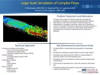
Case Study: Variable-density flow through porous media • Aquifer 600m x 200m fully saturated with fresh water. • Sitting on top, a region of more dense salt water. • Salt water sinks into the aquifer. • Causes complex up-welling and down-welling flows.
Traditional Quiver Plot Animation
Image Base Flow Visualisation Animation
Visualisation Effectiveness (LIC) LIC • Strengths • Dense Coverage. • Spatial Correlation. • Clearly identifies extrema. • Weaknesses • No indicators of direction. • No indicators of magnitude. • Only applicable for steady-state flows.
Visualisation Effectiveness (IBFV) IBFV • Strengths • Dense Coverage. • Spatial/Temporal Correlation. • Clearly identifies extrema. • Identifies motion of extrema. • Strong visual cues for flow direction and magnitude. • Weaknesses • Requires animation. • Care is needed to correctly set texture speeds.
Implementation Comparison LIC Algorithm IBFV Algorithm 1. Warp mesh by field 2. Render with previous texture 3. Overlay next noise texture and blend 4. Copy buffer. • 1. For each pixel • 1.1 Compute forward streamline. • 1.2 Compute backward streamline. • 1.3 Sum pixel intensities • 1.4 Divide by the length • 1.5 Assign result to output pixel.
Extensions to IBFV • Easily extends to advection of multiple textures • Scalar data overlays. movie • Dye injects (particle traces, similar to streaklines). movie • Jittered Grid (similar to quiver plot overlay). movie • Timelines. movie
Computational Aspects • CPU based LIC can be expensive. • Need to implement interpolation. • Streamline tracing for every pixel. • IBFV naturally implemented on GPU • Hardware handles interpolation • Convolution is written in terms of blending functions • Only mesh nodes need be intergrated • LIC IBFV with I(x,t) = I(x)
Future Work • Improve accessibility to researchers. • Integrate into popular tools such as MATLAB.
Thank you! Questions?