Download

1 / 20
200 likes | 205 Views
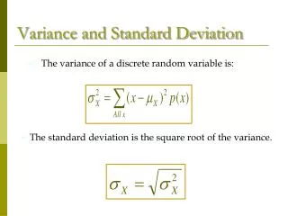
Section 8-6 Testing a Claim About a Standard Deviation or Variance. Key Concept.

E N D
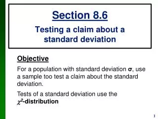
Section 8-6 Testing a Claim About a Standard Deviation or Variance
Key Concept This section introduces methods for testing a claim made about a population standard deviation σ or population variance σ2. The methods of this section use the chi-square distribution that was first introduced in Section 7-5.
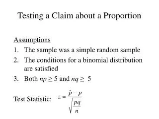
Requirements for Testing Claims About or 2 n= sample size s= sample standard deviation s2 = sample variance = claimed value of the population standard deviation 2 = claimed value of the population variance
Requirements for Testing Claims About or 2 1. The sample is a simple random sample. 2. The population has a normal distribution. (This is a much stricter requirement than the requirement of a normal distribution when testing claims about means.)
Chi-Square Distribution Test Statistic
P-Values and Critical Values for Chi-Square Distribution Use Table A-4. The degrees of freedom = n –1.
Caution The 2 test of this section is not robust against a departure from normality, meaning that the test does not work well if the population has a distribution that is far from normal. The condition of a normally distributed population is therefore a much stricter requirement in this section than it was in Sections 8-4 and 8-5.
Properties of Chi-Square Distribution All values of 2 are nonnegative, and the distribution is not symmetric (see Figure 8-13, following). There is a different distribution for each number of degrees of freedom (see Figure 8-14, following). The critical values are found in Table A-4 using n – 1 degrees of freedom.
Properties of Chi-Square Distribution - cont Chi-Square Distribution for 10 and 20 df Properties of the Chi-Square Distribution Different distribution for each number of df. Figure 8-14 Figure 8-13
Table A-4 Table A-4 is based on cumulative areas from the right (unlike the entries in TableA-2, which are cumulative areas from the left). Critical values are found in Table A-4by first locating the row corresponding to the appropriate number of degrees of freedom (where df = n –1). Next, the significance level is used to determine thecorrect column. The following examples are based on a significance level of = 0.05, but any other significance level can be used in a similar manner.
Table A-4 Right-tailed test: Because the area to the right of the critical value is 0.05, locate 0.05 at the top of Table A-4. Left-tailed test: With a left-tailed area of 0.05, the area to the right of the critical value is 0.95, so locate 0.95 at the top of Table A-4.
Table A-4 Two-tailed test: Unlike the normal and Student t distributions, the critical values in this 2 test will be two different positive values (instead of something like ±1.96 ). Divide a significance level of 0.05 between the left and right tails, so the areas to the right of the two critical values are 0.975 and 0.025, respectively. Locate 0.975 and 0.025 at the top of Table A-4
Example: A common goal in business and industry is to improve the quality of goods or services by reducing variation. Quality control engineers want to ensure that a product has an acceptable mean, but they also want to produce items of consistent quality so that there will be few defects. If weights of coins have a specified mean but too much variation, some will have weights that are too low or too high, so that vending machines will not work correctly (unlike the stellar performance that they now provide).
Example: Consider the simple random sample of the 37 weights of post-1983 pennies listed in Data Set 20 in Appendix B. Those 37 weights have a mean of 2.49910 g and a standard deviation of 0.01648 g. U.S. Mint specifications require that pennies be manufactured so that the mean weight is 2.500 g. A hypothesis test will verify that the sample appears to come from a population with a mean of 2.500 g as required, but use a 0.05 significance level to test the claim that the population of weights has a standard deviation less than the specification of 0.0230 g.
Example: Requirements are satisfied: simple random sample; and STATDISK generated the histogram and quantile plot - sample appears to come from a population having a normal distribution.
Example: Step 1: Express claim as < 0.0230 g Step 2: If < 0.0230 g is false, then ≥ 0.0230 g Step 3: < 0.0230 g does not contain equality so it is the alternative hypothesis; null hypothesis is = 0.0230 g H0: = 0.0230 g H1: < 0.0230 g Step 4: significance level is = 0.05 Step 5: Claim is about so use chi-square
Example: Step 6: The test statistic is The critical value from Table A-4 corresponds to 36 degrees of freedom and an “area to the right” of 0.95 (based on the significance level of 0.05 for a left-tailed test). Table A-4 does not include 36 degrees of freedom, but Table A-4 shows that the critical value is between 18.493 and 26.509. (Using technology, the critical value is 23.269.)
Example: Step 7: Because the test statistic is in the critical region, reject the null hypothesis. There is sufficient evidence to support the claim that the standard deviation of weights is less than 0.0230 g. It appears that the variation is less than 0.0230 g as specified, so the manufacturing process is acceptable.
Recap • In this section we have discussed: • Tests for claims about standard deviation and variance. • Test statistic. • Chi-square distribution. • Critical values.