Download
1 / 51
510 likes | 584 Views
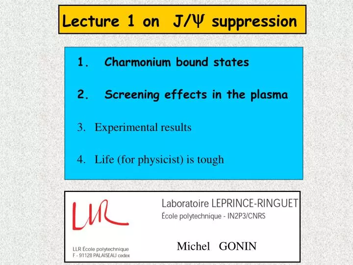
Michel GONIN. Lecture 1 on J/ suppression. 1. Charmonium bound states. 2. Screening effects in the plasma. 3. Experimental results. 4. Life (for physicist) is tough. Heavy Ion Collisions. c. c. Charmonium bound states. Colorless States. V(r). r 0. r. r 0. c. c.

E N D
Michel GONIN Lecture 1 on J/ suppression 1. Charmonium bound states 2. Screening effects in the plasma 3. Experimental results 4. Life (for physicist) is tough
c c Charmonium bound states Colorless States
V(r) r0 r r0 c c Heavy Quark Potential Models
V(r) ½ 2r2- /r r H = p2/2+ V(r) = (1.5/2) GeV = reduced mass and = « free » parameter Hn = Enn Eigen values and vectors
1D Quantum Harmonic Oscillator V = kx2/2 = (k/m)1/2 Etot a =(X+ iP ) /2 a+ =(X- iP ) /2 x -a +a H = h (N + 1/2) Eigen values : Hn= (n + 1/2) hnn = 0,1,2,3,4 … 0 (x) =(m/h)1/2 exp(- mx2/2h) (t)= n cn (n! )-1/2 (a+)n e –i(n+1/2)t0
Hydrogen atom Ek,l = - EI /( k+l )2 k = 1,2,3,4,… 3D Quantum Harmonic Oscillator En = ( k+l + 3/2) h = (n + 3/2) h n=0,1,2,.. V(r) = ½ 2r2 3D HAMILTONIAN H3D = p2/2+ V(r) r2= x2+y2 +z2 p2= px2+py2+pz2
Degenerate States En = (n + 3/2) h E2 = 7h/2 E1 = 5h/2 E0 = 3h/2 l 0 1 2 l = orbital angular momentum
E2 = E0 + 700 MeV E1 = E0 + 350 MeV H3DO E0 l 0 1 2 and = « free » parameter V(r) ½ 2r2- /r
E2 = E0 + 700 MeV E1 = E0 + 350 MeV E0 Why relativistic effects 0 ??
E2 = E0 + 700 MeV E1 = E0 + 350 MeV E0 Why relativistic effects 0 ?? h = 350 MeV and < En> = 4 < T > < Tquark> 80 MeV << mc2 (1500 MeV)
E2 = E0 + 700 MeV E1 = E0 + 350 MeV H3DO E0 l V1(r) = -/r 0 1 2 H=H3DO+V1 V(r) ½ 2r2+ V1(r)
E2 = E0 + 700 MeV E1 = E0 + 350 MeV H3DO E0 l V1(r) = -/r 0 1 2 H=H3DO+V1 V(r) ½ 2r2+ V1(r) Stationary Perturbation Theory (degenerate Eigenvalue) <n , l , m V1n , l , m>
E2 = E0 + 700 MeV 2, 0, 0> 2, 2, m> E1 = E0 + 350 MeV 1, 1, m> H3DO E0 0, 0, 0> l V1(r) = -/r 0 1 2 H=H3DO+V1 V(r) ½ 2r2+ V1(r) Stationary Perturbation Theory (degenerate Eigenvalue) <n , l , m V1n , l , m>
H() = H0 + WH() > = E() () > • En () = En0 + En1 + 2En2 + 3En3 + 4En4 + … • ()> = 0> + 1> + 22> + 3 3 > + … Matrix Eigenvalue Partial Diagonalisation
2, 0, 0> 2, 2, m> 1, 1, m> <0, 0, 0 V1 0, 0, 0> = - 30 ’ 0, 0, 0> <2, 0, 0 V1 2, 0, 0> = - 25 ’ l <1, 1, m V1 1, 1, m> = - 20 ’ 0 1 2 <2, 2, m V1 2, 2, m> = - 16 ’ [L2, V1] = 0
2, 0, 0> 2, 2, m> 1, 1, m> <0, 0, 0 V1 0, 0, 0> = - 30 ’ 0, 0, 0> <2, 0, 0 V1 2, 0, 0> = - 25 ’ l <1, 1, m V1 1, 1, m> = - 20 ’ 0 1 2 <2, 2, m V1 2, 2, m> = - 16 ’ n = 2 l =2 +700 MeV + 702 MeV l =0 n = 2 + 610 MeV n = 1 l =1 +350 MeV + 381 MeV n = 1 n = 0 l =0 E0 E0 n = 0 [L2, V1] = 0
Theory of Fine and Hyperfine Interactions Orbital angular momentum L Spin angular momentum S Overall angular momentum J = S + L H=H3DO+V1 + HFine + HHyperfine Stationary Perturbation Theory ……
l =2 , n = 2 l =2 3770 MeV S=1 n = 2 l =0 3686 MeV l =0 , n = 2 S=0 3654 MeV S=1 J =2 3556 MeV l =1 l =1 , n = 1 n = 1 3526 MeV 3511 MeV S=1 J =0 3417 MeV S=1 l =0 3097 MeV l =0 , n = 0 n = 0 S=0 2980 MeV
l =2 3770 MeV S=1 3686 MeV l =0 S=0 3654 MeV S=1 J =2 3556 MeV l =1 3526 MeV 3511 MeV S=1 J =0 3417 MeV S=1 3097 MeV l =0 S=0 2980 MeV J 0 1 1 0 1 2 J = S + L
3770 3686 3654 3556 3526 3511 3417 3097 2980 0 1 1 0 1 2 MeV ’ J/ J
3770 3686 3654 3556 3526 3511 3417 3097 2980 0 1 1 0 1 2 MeV ’ J/ J
The fundamental state The resonance observed by Crystal Ball… preliminary results …and by E835 in the decay channel:
The state • Crystal ball is the only • experiment which saw an • evidence of this resonance • E760/E835 searched for this • resonance in the energy region: • Ecm=(3570-3660) MeV, in the • decay channel: but no • evidence of a signal was found Crystal Ball • Mass: • Total width:
The resonance E835 is the first experiment which observed the resonance in annihilations
l =2 3770 MeV S=1 3686 MeV l =0 S=0 3654 MeV S=1 J =2 3556 MeV 3526 MeV l =1 3511 MeV S=1 J =0 3417 MeV S=1 3097 MeV l =0 S=0 2980 MeV
Binding Energy (MeV) ’ 40 J/ 670 l =2 3770 MeV S=1 3686 MeV l =0 S=0 3654 MeV S=1 J =2 3556 MeV 3526 MeV l =1 3511 MeV S=1 J =0 3417 MeV S=1 3097 MeV l =0 S=0 2980 MeV
2, 0, 0> 2, 2, m> 1, 1, m> <0, 0, 0 V1 0, 0, 0> = - 30 ’ 0, 0, 0> <2, 0, 0 V1 2, 0, 0> = - 25 ’ l <1, 1, m V1 1, 1, m> = - 20 ’ 0 1 2 <2, 2, m V1 2, 2, m> = - 16 ’ n = 2 l =2 +700 MeV + 702 MeV l =0 n = 2 + 610 MeV n = 1 l =1 +350 MeV + 381 MeV n = 1 n = 0 l =0 E0 E0 n = 0 [L2, V1] = 0 ’ = ? = ?
l =2 + 702 MeV l =0 n = 2 + 610 MeV l =1 + 381 MeV n = 1 l =0 E0 n = 0 E0 = (3/2)h - 30 ’ E1 = (5/2)h - 20 ’ E21 = (7/2)h - 25 ’ E22 = (7/2)h - 16 ’ 381 = h + 10 ’ ’ = 10MeV h = 280MeV 610 = 2 h + 5 ’ 702 = 2 h + 14 ’
VQCD(r) ½ 2r2- /r ( = 15 r0 ’ ) r0 r ’ = 10MeV h = 280MeV r0 = (h/)1/2
’ = 10MeV h = 280MeV r0 = (h/)1/2 VQCD(r) ½ 2r2- /r ( = 15 r0 ’ ) r0 r r0 0.3Fermi « size » of the J/ r02 = (hc)2/c2h
Vem (r) = - (em.hc)/r em = 1/137 0.005 QCD = /hc VQCD(r) ½ 2r2- /r r0 r 0 r VQCD (r) - /r The strong coupling constant : QCD = ?
r0 r ’ = 10MeV h = 280MeV r0 = (h/)1/2 QCD strong interaction QED em 0.005 VQCD (r) -/r QCD = /hc QCD = (15 r0 ’ ) / hc S 0.5
Debye Screening PLASMA Collection of free charged particles A gas is a plasma if it reacts as a « unit » to electric, magnetic , … fields.
Strong interactions QCD • 8 colour gluons ( m=0, spin =1 ) • 1 parameter : gs (flavor independant) gs S
QCD g1 = (r b) q q g5 g2 = (r g) g3 = (b g) q q g4 = (b r) t g5 = (g b) g6 = (g r) QED + + e g7 = (r r + g g - 2b b)/6 g8 = (r r - g g )/2 - - e Strong interactions QCD Quarks : 3 colours ( r , b , g )
Electroweak Strong (QCD) 10 GeV 90 GeV 1 GeV QCD S
Strong interactions QCD Gluon coupling -> « anti-screening » effects screening anti-screening for « small » distances, QCD 0
Strong interactions QCD QCD screening effects asymptotic freedom
x Debye Screening PLASMA “Test charge” • Collective response to charge fluctuation (local surplus) reducing the “long” range nature of the interaction But every individual charge is indeed a local fluctuation statistical effects …… equilibrium
Spatial density of charges : Poisson equation : KT e Solution : = potentiel T = temperature (Boltzmann) Interaction « energy » Thermal kinetic energy kD-1=D = Debye screening radius
In an electromagnetic plasma, the potential of a charge is screened by the field of the electrons that surround it n0 = density of electrons in the plasma
In an electromagnetic plasma, the potential of a charge is screened by the field of the electrons that surround it n0 = density of electrons in the plasma In a QGP, the strong colored field will be screened. e2(Gauss system) aQCD ~ 1 kT ~ 200 MeV n0n = 3.6 T3(Stefan-Boltzmann law) n = 28.8 106 MeV3
c c Debye Screening PLASMA x x
Debye Screening PLASMA x x Debye Screening no more bound states
q q V r T = Tc STRONG INTERACTIONS QCD PREDICTION
quarkonia q q Lattice QCD ’ T > Tc = 0 Signals for the Deconfinement Successive (vs. temperature) melting for the quarkonia Satz et al.