Download

1 / 50
500 likes | 592 Views
Previous Lecture: Sequence Database Searching. This Lecture. Introduction to Biostatistics and Bioinformatics Distributions. By Judy Zhong Assistant Professor Division of Biostatistics Department of Population Health Judy.zhong@nyumc.org.

E N D
This Lecture Introduction to Biostatistics and Bioinformatics Distributions By Judy Zhong Assistant Professor Division of Biostatistics Department of Population Health Judy.zhong@nyumc.org
Last lecture defined probability and introduced some basic tools used in working with probabilities This lecture discusses specific probability models Three specific probability distributions (models) Binomial distribution Poisson distribution Normal distribution Introduction
A random variable is a function that assigns numeric values to different events in a sample space NOTE: (1) Randomness; (2) Numeric values Example 1: Randomly select a student from a class. X=student’s number of siblings. X could be 0, 1, 2 … Example 2: Randomly select a student from a class. X=student’s height. X could be any value bigger than 0 Random variables
A random variable for which there exists a discrete set of numeric values is a discrete random variable A random variable whose possible values cannot be enumerated is a continuous random variable Two types of random variables
A probability distribution function is a mathematical relationship, or rule, that assigns to any possible value r of a discrete random variable X the probability Pr(X=r). Probability distribution function
The expected value (expectation) of a discrete random variable is defined as Where x_i’s are the values the random variable X assumes with positive probability The sum is over all the R possible values. R may be finite (e.g., binomial distribution) or infinite (e.g., Poisson distribution) Expectation represents “average” value of the random variable Expected value (expectation) of a discrete random variable
The variance of a discrete random variable is defined by The standard deviation of a random variable is defined by Variance (population variance) of a discrete random variable
Common structure for binomial distribution: A sample of n independent trials Each trial can have only two possible outcomes, which are denoted as “success” and “failure” (the term “success” is used in a general way, without specific meaning) The probability of a success at each trial is assumed to be the same, with probability p (hence the probability of failure is 1-p=q) Let random variable: X=number of successes among n trails An experiment (for binomial distribution)
Here we concentrate on counting the number of neutrophils of 5 white blood cells. Assume that the probability that a cell is neutrophils is 0.6 number of trials n=5 “success”=“one cell being neutrophils” Pr(“success”)=p=0.6 X=number of successes among 5 How to fit a real problem into binomial structure
There are 5 white cells, each of cell is either neutrophils (N) or other (O). What is the probability that the 2nd and the 5th cells considered will be neutrophils and the remaining cells are non-neutrophils? That is, what is the probability of outcome “ONOON” Assume that the outcomes for different cells are independent. Using multiplication law of probability, Think about this question: What is the probability that any 2 cells out of 5 will be neutrophils? How to calculate the probability of an outcome from binomial structure
Possible outcomes for 2 neutophils of 5 cells: NNOOO, ONNOO, … How many such outcomes? Then the probability of obtaining 2 neutrophils in 5 cells is: Combination plays an role …
Let X=number of success in n statistically independent trials, where the probability of success is p The distribution of random variable X is known as the binomial distribution and has probability distribution function given by Binomial distribution
Table 1 in the Appendix: for n=2, 3, …, 20 and p=0.05, 0.10, …, 0.50 Using binomial tables
Result: The expected value and the variance of a binomial distribution are np and np(1-p), respectively Expected value and variance of the binomial distribution
Look at a special case of binomial random variable with n=1 and p. That is, conduct only one trial, X=1 if success and X=0 if failure: Pr(X = 1) =p Pr(X = 0) = 1 − p = q Expectation of X: E(X)=1*p+0*q=p Variance of X: Var(X)=(1^2*p+0^2*q)-p^2=p*(1-p)=pq Bernoulli distribution
Conduct n independent trials, each trail having outcome either success or failure For each trail, probability of success is p X=number of successes among n trials. It is known that the distribution of X is binomial distribution with n and p Now define the outcome of the ith trial as Xi (Xi=1 if success and Xi=0 if failure), then Write binomial random variable in terms of bernoulli random variables
Fact 1: Fact 2: For any i, E(Xi)=p and Var(Xi)=pq Then (1) , where the first equality always holds (2) , where the first equality only holds for independent variables Proof of expectation and variable of binomial variable
The Poisson distribution is the second most frequently used discrete distribution after the binomial distribution. Poisson distribution is usually associated with rare events (for example, rare diseases) Poisson distribution for rare events
number of deaths attributed to typhoid fever over a year Assuming the probability of a few death from typhoid fever in any one day is vey small and the number of cases reported in any two days are independent random variables, then the number of deaths over a 1-year period will follow a Poisson distribution number of bacterial colonies growing on an agar plate. Suppose we have a 100-cm^2 agar plate. The probability of finding any bacterial colonies on a small area is very small, and the events finding bacterial colonies at any two areas are independent. The number of bacterial colonies over the entire agar plate will follow a Poisson distribution Examples
The probability of k events occurring for a Poisson distribution with parameter is Poisson distribution
For =0.5, 1.0, 1.5, …, 20.0 Use Poisson table (Table 2 in the Appendix)
Result: For a Poisson distribution with parameter , the mean and variance are both equal to Expectation and variance of a Poisson random variable
u = 2.5 u = 7.5 u = 15
Binomial when n is large and p is very small • X~bin(n, p) • E(X) = np • Var(X) = np(1-p)=npq • If n is large and p is very small, 1-p = q ≈ 1 • Then np ≈ npq • That is, E(X)≈ Var(X)
For discrete variable, probability distribution gives the probability of each value that the variable takes on. Can we have the same distribution for continuous variable? The answer is: NO For a continuous DBP, the probabilities of specific blood-pressure measurement values such that 117.341123 are 0, and thus the concept of a probability distribution (probability mass) function cannot be used Instead, we speak in terms of the probability that blood pressure X falls within a range of values, for examples, ranges 90≤X<100, or a≤X<b Probability that a continuous random variable falls in range [a, b]
The probability density function (pdf) of the random variable X is a function such that the area under the density function curve between any two points a and b is equal to the probability that the random variable X falls between a and b. Thus, the total area under the density function curve over the entire range of possible values for the random variable is 1 The pdf has large values in regions of high probability and small values in regions of low probability Probability density function
As discussed earlier, for a continuous random variable X, Pr(X=x)=0 for any specific value x Generally, a distinction is not made between probabilities such as Pr(X<x) and Pr(X≤x), Pr(a≤X≤b) and Pr(a<X<b) when X is a continuous The pdf of a continuous random variable X is usually denoted as f(x) In mathematics, the probability of X in interval [a, b] is equal to the integration (area) of its pdf over [a,b], that is Some remarks
The expectation of a continuous random variable X, denoted by E(X), or , is the average value taken on by the random variable The variance of a continuous random variable X, denoted by Var(X) or , is the average squared distance of each value of the random variable from its expectation, which is given by . The standard deviation, or , is the square root of the variance, that is, Expectation and variance
Normal distribution is also called Gaussian distribution, after the well-known mathematician Karl Gauss (1777-1855, “the Prince of Mathematicians“) Normal distribution is very useful Many variables are normally distributed Many other distributions an be made approximately normal by transformation Normal distribution is as approximation of other distribution such as binomial distribution and Poisson distribution Most statistical methods considered in this text are based on normal distribution Normal distribution
The normal distribution is defined by its pdf, which is given as for some parameters and The pdf of normal distribution • : Mean • : Standard deviation • = 3.14159 • e = 2.71828
Bell-shaped, symmetric with mode and center at A point of inflection is a point at which the slope of the curve directions. Image you are skiing on a mountain An example of Normal pdf
In the graph, 2>1 Location is measured by
In the graph, 2>1 Spread is measured by σ2
A normal distribution with mean 0 and variance 1 is called a standard normal distribution. Denoted as N(0, 1) In the following, we will examine the standard normal distribution N(0, 1) in detail We will see that any information concerning a general normal distribution N(, σ2) can be obtained from appropriate manipulations of an N(0,1) distribution Standard normal distribution N(0, 1)
It can be shown that about 68% of the area under the standard normal density lies between -1 and +1, about 95% of the area lies between -2 and +2, and about 99% lies between -2.5 and +2.5 NOTE: You will see that, more precisely, Pr(-1<x<1)=0.6827, Pr(-1.96<X<1.96)=0.95, Pr(-2.576<X<2.576)=0.99 Properties of the standard normal N(0, 1)
The cumulative distribution function (cdf) for a standard normal distribution is denoted by (x)=Pr(X≤x), where X~N(0,1) The symbol ~ is used as shorthand for the phase “is distributed as.” Thus X~N(0,1) means that the random variable X is distributed as an N(0,1) distribution Generally, X~N(, σ2) means X is distributed as N(, σ2) Some notations
From the symmetry property of the N(0,1), (-x)=Pr(X≤-x)=Pr(X≥x)=1-Pr(X≤x)=1-(x) Example 5.12: Find P(X≤-1.96) if X~N(0,1) Using symmetry properties of N(0,1)
Example 5.13: Find Pr(-1≤X≤1.5) if X~N(0,1) Solution: Pr(-1≤X≤1.5) =Pr(X≤1.5)-Pr(X≤-1) =Pr(X≤1.5)-Pr(X≥1)=0.9332-0.1587=0.7745 (NOTE: The best way to work on such problems is to draw a graph!) Pr(a≤X≤b)=Pr(X≤b)-Pr(X≤a)
The (100u)th percentile of N(0,1) is denoted by zu such that, Pr(X<zu)=u, where X~N(0,1) The (100u)th percentile
Example 5.18: Compute z0.975 ,z0.95 ,z0.5 and z0.025 (1) 1.96; (2) 1.645; (3) 0; (4) -1.96 Example of finding percentiles
Now we have become familiar with N(0,1), but we want to work on any general normal N(, σ2) Example 5.20 (Hypertension): Suppose a mild hypertensive is defined as a person whose DBP is between 90 and 100 mm Hg inclusive, and the subjects are 35- to 40-year-old men whose blood pressure are normally distributed with mean 80 and variance 144. What is the probability that a randomly selected person from this population will be a mild hypertensive? This question can be stated more precisely: If X~N(80, 144), then what is Pr(90<X<100)? Now: from N(, σ2) to N(0,1)
How to standardize the normal distribution? Then Z has a standard normal distribution, Z ~ N(0, 1)
IF X~ N(, σ2) and Z=(X-µ)/, then Z~N(0,1) Then where the last two terms can be found from column A in normal table Standardization
Example 5.20 (Hypertension example continued): If X~N(80, 12^2), what is Pr(90<X<100)? Solution: Use standardization for many problems
Next Lecture: Estimation I Point Estimate Interval Estimate