Download

1 / 62
620 likes | 813 Views
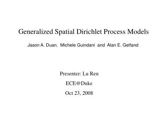
Double Dirichlet Process Mixtures. Sanjib Basu. Northern Illinois University and Rush University Medical Center. Siddhartha Chib. Washington University, St. Louis. Dirichlet process mixtures are active research areas Dirichlet mixtures are it!

E N D
Double Dirichlet Process Mixtures Sanjib Basu Northern Illinois University and Rush University Medical Center Siddhartha Chib Washington University, St. Louis
Dirichlet process mixtures are active research areas • Dirichlet mixtures are it! • The flexibility of DPM models supported its huge popularity in wide variety of areas of application. • DPM models are general and can be argued to have less structure. • Double Dirichlet Process Mixtures add a degree of structure, possibly at the expense of some degree of flexibility, but possibly with better interpretability in some cases • We discuss applications (and limitations) of these semiparametric double mixtures • We compare fit-prediction duality with competing models
Other DP extensions • Double Dirichlet process mixtures are a subclass of dependent Dirichlet Process mixtures (MacEachern 1999,……) • Double DP mixture are different from Hierarchical Dirichlet Processes (The et al. 2006 ) • Double DPM is simply independent DPMS
Motivating Example 1 • Luminex measurements on two biomarker proteins from n=156 Patients • IL-1β protein • C-reactive protein • The biological effects of these two proteins are thought to be not (totally) overlapping.
Two Biomarkers (y1 and y2) • Usual DP mixture of normals (Ferguson 1983,…..) Questions • Should we model the two biomarkers jointly? • Should we cluster the patients based on both biomarkers jointly? • The biomarkers may operate somewhat independently.
Double DP mixtures • Equicorrelation – corr(y1i, y2i) are assumed to be the same for all i=1,…,n • Clustering based on biomarker 1 and based on biomarker 2 can be different
Motivating Example 2: Interrater Agreement • Agreement between 2 Raters (Melia and Diener-West 1994) • Each rater provides an ordinal rating on a scale of 1-5 (lowest to highest invasion)of the extent to which tumor has invaded the eye,n=885
Interrater agreement • Kottas, Muller, Quintana (2005) analyzed these data using a flexible DP mixture of Bivariate probit ordinal model which modeled the unstructured joint probabilities prob(Rater 1=i and Rater2 = j), i=1,…,5, j=1,…,5 • One way to quantify interrrater agrrement is to measure departure from the structured model of independence • We consider a (mixture of) Double DP mixtures model here which provides separate DP structures for the two raters. We then measure ``agreement’’ from this model.
Motivating Example 3 • Mixed model for longitudinal data • It is common to assume (Bush and MacEachern 1996) • Modeling the error covariance i or the error variance (if i =diag(2i)) extends the normal distribution assumption to normal scale mixtures (t, Logistic,…)
Putting the two together • One way to combine these two structures is • Do we expect the random effects bi appearing in the modeling the mean and the error variances to cluster similarly? • The error variance model often is used to extend the distributional assumption.
Double DPM • I will discuss • Fitting • Applicability • Flexibility • Limitations of such double semiparametric mixtures • I will also compare these models with usual DP models via predictive model comparison criteria
Dirichlet process • Dirichlet Process is a probability measure on the space of distributions (probability measures) G. • G ~ Dirichlet Process (G0), where G0 is a probability • Dirichlet Process assigns positive mass to every open set of probabilities on support(G0) • Conjugacy:Y1,…., Yn ~ i.i.d. G, (G) = DP( G0)Then Posterior (G|Y) ~ DP( G0 + nFn) where Fn is the empirical distn. • Polya Urn Scheme
Stick breaking and discreteness • G~ DP( G0) impliesG is almost surely discrete
Bayes estimate from DP • The discrete nature of a random G from a DP leads to some disturbing features, such as this result from Diaconis and Freedman (1986) • Location model yi = + i, i=1,…n • has prior (), such as a normal prior • 1,…, n ~ i.i.d. GG ~ DP(G0) - symmetrizedG0= Cauchy or t-distn • Then the posterior mean is an inconsistent estimate of
Dirichlet process mixtures (DPM) • If we marginalize over i, we obtain a semiparametric mixturewhere the mixing distribution G is random and follows DP(G0)
DPM - clusters • Since G is almost surely discrete, 1,…,nform clusters • 1= 5 = 8 1unique • 2= 3 = 4= 6= 7 2uniqueetc. • The number of clusters, and the clusters themselves, are random.
DPM – MCMC • The Polya urn/marginalized sampler (Escobar 1994, Escobar & West 1995) samples ione-at-a-time from(i | -i, data) • Improvements, known as collapsed samplers, are proposed in MacEachern (1994, 1998) where, instead of sampling i, only the cluster membership of iare sampled. • For non-conjugate DPM (sampling density f(yi |i ) and base measure G0 are not conjugate), various algorithms have been proposed.
Finite truncation and Blocked Gibbs • With this finite truncation, it is now a finite mixture model with stick-breaking structure on qj • (1,....,n) and(q1,....,qM) can be updated in blocks (instead of one-at-time as in Polya Urn sampler) which may provide better mixing
Comments • In each iteration, the Polya urn/marginal sampler cycles thru each observation, and for each, assigns its membership among a new and existing clusters. • The Poly urn sampler is also not straightforward to implement in non-linear (non-conjugate) problems or when the sample size n may not be fixed. • For the blocked sampler, on the other hand, the choice of the truncation M is not well understood.
Model comparison in DPM models • Basu and Chib (2003) developed Bayes factor/ marginal likelihood computation method for DPM. • This provided a framework for quantitativecomparison of DPM with competing parametric and semi/nonparametric models.
Marginal likelihood of DPM • Based on the Basic marginal identity (Chib 1995)log-posterior()=log-likelihood() + log-prior() - log-marginallog-marginal = log-likelihood(*) + log-prior(*) – log-posterior(*) • The posterior ordinate of DPM is evaluated via prequential conditioning as in Chib (1995) • The likelihood ordinate of DPM is evaluated from a (collapsed) sequential importance sampler.
Double Dirichlet process mixtures (DDPM) • Marginalization obtains a double semiparametric mixturewhere the mixing distributions Gand G are random
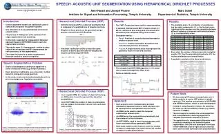
A simpler model: normal means only • We generate n=50 (i,i) means and then (yi1,yi2) observations from this Double-DPM model
Single DPM in the bivariate mean vector Double DPM in mean components
Model fitting • We fitted the Double DPM and the Bivariate DPM models to these data. • The Double DPM model can be fit by a two-stage Polya urn sampler or a two-stage blocked Gibbs sampler. • “Collapsing” can become more difficult.
Wallace (asymmetric) criterion for comparing two clusters/partitions • Let S be the number of mean pairs which are in the same cluster in a MCMC posterior draw and also in the true clustering. • Let nk, k=1,..K be the number of means in cluster Ck in the MCMC draw. • Then the Wallace asymmetric criterion for comparing these two clusters is
Measurements on two biomarker proteins by Luminex panels • Frozen parafin embedded tissues, pre and post surgery • Luminex panel • Nodal involvement
Two biomarker proteins • The bivariate DPM • vs the Double DPM
log CPO = log f(yi| y-i) LPML = log f(yi| y-i) Double DP = -1498.67 Bivariate DP= -1533.01
Model comparison • I prefer to use marginal likelihood/ Bayes factor for model comparison. • The DIC (Deviance Information Criterion) , as proposed in Spiegelhalter et al. (2002) can be problematic for missing data/random-effects/mixture models. • Celeux et al. (2006) proposed many different DICs for missing data models
DIC3 • I have earlier considered DIC3 (Celeux et al. 2006, Richardson 2002) in missing data and random effects models which is based on the observed likelihood • The integration over the latent parameters often has to be obtained numerically. • This is difficult in the present problem
DIC9 • I am proposing to use DIC9 which is similar to DIC3 but is based on the conditional likelihood
Convergence rate results: Ghosal and Van Der Vaart (2001) • Normal location mixturesModel:Yi~ i.i.d. p(y) = (y-)dG(), i=1,…,nG ~ DP(G0), G0 is NormalTruth:p0(y) = (y-)dF() • Ghosal and Van Der Vaart (2001): Under some regularity conditions,Hellinger distance(p, p0) 0 “almost surely” at the rate of (log n)3/2/n
Ghosal and Van Der Vaart (2001): results contd. • Bivariate DP location-scale mixture of normalsYi~ i.i.d. p(y) = (y-)dH(,), i=1,…,n H~DP(H0) • Ghosal and Van Der Vaart (2001): If H0 is Normal {a compactly supported distn}, then the convergence rate is(log n)7/2/n • Double DP location-scale mixture of normalsYi~ i.i.d. p(y) = (y-)dG() dG(), i=1,…,n G ~DP(G0), G ~DP(G0) • Ghosal and Van Der Vaart (2001): If G0 is Normal, G0 is compactly supported and the true densityp0(y) = (y-)dF1() dF2() is also a double mixture, then Hellinger distance(p, p0) 0 at the rate of (log n)3/2/n
Interrater data • Agreement between 2 Raters (Melia and Diener-West 1994) • Each rater provides an ordinal rating on a scale of 1-5 (lowest to highest invasion)of the extent to which tumor has invaded the eye,n=885
DPM multivariate ordinal model • Kottas, Muller and Quintana (2005)
Interrater agreement • The objective is to measure agreement between raters beyond what is possible by chance. • This is often measured by departure from independence, often specifically in the diagonals • Polychoric correlation of the latent bivariate normal Z has been used as a measure of association. • ………………… of the latent bivariate normal mixtures???
Latent class model (Agresti & Lang 1993) • C latent classes • Ratings of the two raters within a class are independent
Mixtures of Double DPMs • For each latent class, we model pc1j and pc2k by two separate univariate ordinal probit DPM models
Computational issue • The ``sample size’’ nc in latent group c is not fixed. This causes problem for the polya-urn/marginal sampler which works with fixed sample size • Do, Muller, Tang (2005) suggested a solution to this problem by jointly sampling the latent il =(il,il2) and the latent rating class membership i.